Imaging and Deconvolution

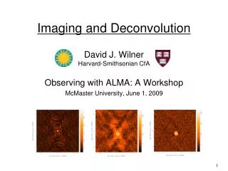
Imaging and Deconvolution David J. Wilner (Harvard-Smithsonian Center for Astrophysics)

References • Thompson, A.R., Moran, J.M., Swensen, G.W. 2004 “Interferometry and Synthesis in Radio Astronomy”, 2nd edition (Wiley-VCH) • previous Synthesis Imaging Workshop proceedings • Perley, R.A., Schwab, F.R., Bridle, A.H. eds. 1989 ASP Conf. Series 6 “Synthesis Imaging in Radio Astronomy” (San Francisco: ASP) • Ch. 6 Imaging (Sramek & Schwab) and Ch. 8 Deconvolution (Cornwell) • www.aoc.nrao.edu/events/synthesis • lectures by Cornwell 2002 and Bhatnagar 2004, 2006 • IRAM Interferometry School proceedings • www.iram.fr/IRAMFR/IS/IS2008/archive.html • Ch. 13 Imaging Principles and Ch. 16 Imaging in Practice (Guilloteau) • lectures by Pety 2004-2012 • many other lectures and pedagogical presentations are available • ALMA primer, ATNF, CARMA, ASIAA, e-MERLIN, … • Fourteenth Synthesis Imaging Workshop

Visibility and Sky Brightness • V(u,v), the complex visibility function, is the 2D Fourier transform of T(l,m), the sky brightness distribution (for incoherent source, small field of view, far field, etc.) [for derivation from van Cittert-Zernike theorem, see TMS Ch. 14] • mathematically T(l,m) • u,vare E-W, N-S spatial frequencies [wavelengths] • l,mare E-W, N-S angles in the tangent plane [radians] • (recall ) • Fourteenth Synthesis Imaging Workshop

The Fourier Transform • Fourier theory states and any well behaved signal (including images) can be expressed as the sum of sinusoids Jean Baptiste Joseph Fourier 1768-1830 signal 4 sinusoids sum • the Fourier transform is the mathematical tool that decomposes a signal into its sinusoidal components • the Fourier transform contains all of the information of the original signal

The Fourier Domain • acquire some comfort with the Fourier domain • in older texts, functions and their Fourier transforms occupy upper and lower domains, as if “functions circulated at ground level and their transforms in the underworld” (Bracewell 1965) • some properties of the Fourier transform adding scaling shifting convolution/multiplication Nyquist-Shannon sampling theorem

Visibilities • each V(u,v) contains information on T(l,m)everywhere, not just at a given (l,m) coordinate or within a particular subregion • each V(u,v) is a complex quantity • expressed as (real, imaginary) or (amplitude, phase) T(l,m) V(u,v) phase V(u,v)amplitude

Example 2D Fourier Transforms V(u,v) amplitude T(l,m) narrow features transform into wide features (and vice-versa) elliptical Gaussian δ function elliptical Gaussian constant Gaussian Gaussian

Example 2D Fourier Transforms V(u,v) amplitude T(l,m) sharp edges result in many high spatial frequencies uniform disk Bessel function

Amplitude and Phase T(l,m) V(u,v) amplitude V(u,v) phase • amplitude tells “how much” of a certain spatial frequency • phase tells “where” this spatial frequency component is located

The Visibility Concept • visibility as a function of baseline coordinates (u,v) is the Fourier transform of the sky brightness distribution as a function of the sky coordinates (l,m) • V(u=0,v=0) is the integral of T(l,m)dldm= total flux density • since T(l,m) is real, V(-u,-v) = V*(u,v) • V(u,v) is Hermitian • get two visibilities for one measurement

The Visibility Concept

Aperture Synthesis Basics • idea: sample V(u,v) at enough (u,v) points using distributed small aperture antennas to synthesize a large aperture antenna of size (umax,vmax) • one pair of antennas = one baseline = two (u,v) samples at a time • N antennas = N(N-1) samples at a time • use Earth rotation to fill in (u,v) plane over time (Sir Martin Ryle, 1974 Nobel Prize in Physics) • reconfigure physical layout of N antennas for more samples • observe at multiple wavelengths for (u,v) plane coverage, for source spectra amenable to simple characterization (“multi-frequency synthesis”) • if source is variable, then be careful Sir Martin Ryle 1918-1984

Examples of Aperture Synthesis Telescopes (for Millimeter Wavelengths) Jansky VLA SMA IRAM PdBI ATCA ALMA CARMA

An Example of (u,v) plane Sampling VEX configuration of 6 SMA antennas, ν = 345 GHz, dec = +22 deg

An Example of (u,v) plane Sampling EXT configurations of 7 SMA antennas, ν = 345 GHz, dec = +22 deg

An Example of (u,v) plane Sampling COM configurations of 7 SMA antennas, ν = 345 GHz, dec = +22 deg

An Example of (u,v) plane Sampling 3 configurations of SMA antennas, ν = 345 GHz, dec = +22 deg

Implications of (u,v) plane Sampling • samples of V(u,v) are limited by number of antennas and by Earth-sky geometry • outer boundary • no information on smaller scales • resolution limit • inner hole • no information on larger scales • extended structures invisible • irregular coverage between boundaries • sampling theorem violated • information missing

Inner and Outer (u,v) Boundaries T(l,m) V(u,v) phase V(u,v) phase V(u,v)amplitude V(u,v)amplitude T(l,m)

xkcd.com/26/

Formal Description of Imaging • sample Fourier domain at discrete points • Fourier transform sampled visibility function • apply the convolution theorem where the Fourier transform of the sampling pattern is the “point spread function” the Fourier transform of the sampled visibilities yields the true sky brightness convolved with the point spread function radio jargon: the “dirty image” is the true image convolved with the “dirty beam”

Dirty Beam and Dirty Image S(u,v) s(l,m) “dirty beam” TD(l,m) “dirty image” T(l,m)

Dirty Beam Shape and N Antennas 2 Antennas, 1 Sample

Dirty Beam Shape and N Antennas 7 Antennas, 10 min

Dirty Beam Shape and N Antennas 7 Antennas, 2 x 10 min

Dirty Beam Shape and N Antennas 7 Antennas, 1 hour

Dirty Beam Shape and N Antennas 7 Antennas, 3 hours

Dirty Beam Shape and N Antennas 7 Antennas, 8 hours

Calibrated Visibilities: What’s Next? • analyze directly V(u,v) samples by model fitting • goodfor simple structures, e.g. point sources, symmetric disks • sometimes for statistical descriptions of sky brightness • visibilities have very well defined noise properties • recover an image from the observed incomplete and noisy samples of its Fourier transform for analysis • Fourier transform V(u,v) to get TD(l,m) • difficult to do science with the dirty image TD(l,m) • deconvolves(l,m) from TD(l,m) to determine a model of T(l,m) • work with the model of T(l,m)

Some Details of the Dirty Image • “Fourier transform” • Fast Fourier Transform (FFT) algorithm is much faster than simple Fourier summation, O(NlogN) for 2Nx 2N image • FFT requires data on a regularly spaced grid • aperture synthesis does not provide V(u,v) on a regularly spaced grid, so… • “gridding” used to resample V(u,v) for FFT • customary to use a convolution method • special (“spheroidal”) functions that minimize smoothing and aliasing

Antenna Primary Beam Response T(l,m) • antenna response A(l,m) is not uniform across the entire sky • main lobe = “primary beam” fwhm ~ λ/D • response beyond primary beam can be important (“sidelobes”) • antenna beam modifies the sky brightness distribution • T(l,m) T(l,m)A(l,m) • can correct with division by A(l,m) in the image plane • large source extents require multiple pointings of antennas = mosaicking A(l,m) D SMA 6 m 345 GHz ALMA 12 m 690 GHz

Imaging Decisions: Pixel Size, Image Size • pixel size • satisfy sampling theorem for longest baselines • in practice, 3 to 5 pixels across main lobe of dirty beam to aid deconvolution • e.g. at 870 μm with baselines to 500 meters  pixel size < 0.1 arcsec • CASA “cell” size • image size • natural choice is often the full extent of the primary beam A(l,m) • e.g. SMA at 870 μm, 6 meter antennas  image size 2 x 35 arcsec • if there are bright sources in the sidelobes of A(l,m), then the FFT will alias them into the image  make a larger image (or equivalent) • CASA “imsize”

Imaging Decisions: Visibility Weighting • introduce weighting function W(u,v) • modifies sampling function • S(u,v) S(u,v)W(u,v) • changes s(l,m), the dirty beam shape • natural weight • W(u,v) = 1/σ2 in occupied (u.v) cells, where σ2 is the noise variance, and W(u,v) = 0 everywhere else • maximizes point source sensitivity • lowest rms in image • generally gives more weight to short baselines (low spatial frequencies), so angular resolution is degraded

Dirty Beam Shape and Weighting • uniform weight • W(u,v) is inversely proportional to local density of (u,v) points • sum of weights in a (u,v) cell = const (and 0 for empty cells) • fills (u,v) plane more uniformly and dirty beam sidelobes are lower • gives more weight to long baselines (high spatial frequencies), so angular resolution is enhanced • downweights some data, so point source sensitivity is degraded • can be trouble with sparse sampling: cells with few data points have same weight as cells with many data points

Dirty Beam Shape and Weighting • robust (Briggs) weight • variant of uniform that avoids giving too much weight to (u.v) cells with low natural weight • software implementations differ • e.g. SN is natural weight of cell Sthresh is a threshold high threshold natural weight low threshold uniform weight • an adjustable parameter allows for continuous variation between maximum point source sensitivity and resolution

Dirty Beam Shape and Weighting • tapering • apodize(u,v) sampling by a Gaussian t= adjustable tapering parameter • like smoothing in the image plane (convolution by a Gaussian) • gives more weight to short baselines, degrades angular resolution • downweights some data, so point source source sensivitity degraded • may improve sensitivity to extended structure sampled by short baselines • limits to usefulness

Weighting and Tapering: Image Noise natural 0.59x0.50 rms=1.0 robust=0 0.40x0.34 rms=1.3 robust=0 + taper to 0.59x0.50 rms=1.2 natural + taper to 1.5x1.5 rms=1.4 uniform 0.35x0.30 • rms=2.1

Weighting and Tapering: Summary • imaging parameters provide a lot of freedom • appropriate choices depend on science goals

Beyond the Dirty Image: Deconvolution • to keep you awake at night •  an infinite number of T(l,m) compatible with sampled V(u,v), with “invisible” distributions R(l,m) where s(l,m) * R(l,m) = 0 • no data beyond umax,vmax unresolved structure • no data within umin,vmin limit on largest size scale • holes in between  synthesized beam sidelobes • noise  undetected/corrupted structure in T(l,m) • no unique prescription for extracting optimum estimate of T(l,m) • deconvolution • uses non-linear techniques to interpolate/extrapolate samples of V(u,v) into unsampled regions of the (u,v) plane • aims to find a sensible model of T(l,m) compatible with data • requires a priori assumptions about T(l,m) to pick plausible “invisible” distributions to fill unmeasured parts of the Fourier plane

Deconvolution Algorithms • an active research area, e.g. compressive sensing methods • clean: dominant deconvolution algorithm in radio astronomy • a priori assumption: T(l,m) is a collection of point sources • fit and subtract the synthesized beam iteratively • original version by Högbom (1974) purely image based • variants developed for higher computational efficiency, model visibility subtraction, to deal better with extended emission structure, etc. • maximum entropy: a rarely used alternative • a priori assumption: T(l,m) is smooth and positive • define “smoothness” via a mathematical expression for entropy, e.g. Gull and Skilling (1983), find smoothest image consistent with data • vast literature about the deep meaning of entropy as information content

Imaging and Deconvolution