Download

1 / 24
360 likes | 599 Views
Surface Exchange Processes. SOEE3410 : Lecture 3 Ian Brooks. Turbulence. The exchange of energy and trace gases at the surface is achieved almost entirely via turbulent mixing .

E N D
Surface Exchange Processes SOEE3410 : Lecture 3 Ian Brooks
Turbulence • The exchange of energy and trace gases at the surface is achieved almost entirely via turbulent mixing. • Wind is generated on large scales by spatial differences in atmospheric pressure (ultimately resulting from radiative heating/cooling) • Kinetic energy of wind is dissipated at small scales by friction (and ultimately as heat) SOEE3410 : Atmosphere and Ocean Climate Change
Friction: mechanical generation of turbulence Flow over rough surface / obstacles Small perturbations of the flow act as obstacles to the surrounding flow Shear in the flow can result in instability & overturning Turbulence results in a wind speed profile that is close to logarithmic Sources of Turblence z Wind speed SOEE3410 : Atmosphere and Ocean Climate Change
Convection: heating of air near the surface (or cooling of air aloft) increases (decreases) its density with respect to the air around it, so that it becomes buoyant. SOEE3410 : Atmosphere and Ocean Climate Change
Large Eddy Model simulation of convective mixing SOEE3410 : Atmosphere and Ocean Climate Change
Turbulent Fluxes • The turbulent flux of some quantity x (momentum, heat, CO2,…) is defined as: Flux of x = 1 (w′1x′1 + w′2x′2 + …w′Nx′N) N = w′x′ Where w′N = wN – w And an overbar signifies an average SOEE3410 : Atmosphere and Ocean Climate Change
For example, the wind stress at the surface (the vertical flux of horizontal momentum) is where is air density, and U the wind speed. More strictly it is where u is the wind component in the direction of the mean wind direction and v the component perpendicular to the mean wind. The wind stress is frequently represented by the friction velocity SOEE3410 : Atmosphere and Ocean Climate Change
Flux Parameterizations • Measurement of turbulent fluxes is possible only on small scales, using expensive instrumentation. • Large-scale climate models do not include small-scale processes such as turbulence directly; they must parameterize the effects of turbulence in terms of large-scale mean quantities: • Mean wind speed • Temperature difference between surface and a given altitude • Within the surface layer turbulent fluxes are almost constant with altitude SOEE3410 : Atmosphere and Ocean Climate Change
z U U = mean wind speed Z = altitude k = von-Karman’s constant (0.4) zo = the roughness length – a measure of the roughness of the surface; the altitude at which the mean wind speed falls to zero. u* = the friction velocity – a measure of how variable (turbulent) the wind speed is in the direction of the mean wind. = (w′u′)½ Wind speed SOEE3410 : Atmosphere and Ocean Climate Change
Similar relationships describe the shape of vertical profiles of scalar quantities such as temperature, water vapour concentration, and gas concentrations. e.g: Where Ts is the surface temperature and T* is a measure of how variable the temperature is. The sensible heat flux, QH is given by: where is the air density and Cp is the specific heat capacity of air at constant pressure. SOEE3410 : Atmosphere and Ocean Climate Change
The vertical flux F of any quantity, , is assumed to be driven by its vertical gradient, approximated by the difference in value between two levels – usually the surface and z. Where UT represents a transport velocity. Note ‘-’ sign: direction of flux is down-gradient. The transport velocity is usually parameterized as a function of some measure of turbulence. e.g. Where Uz is the mean wind speed at height z, and CD is a bulk transfer coefficient. Bulk Transfer Schemes SOEE3410 : Atmosphere and Ocean Climate Change
Using u* as a measure of the surface stress associated with drag: For momentum transfer, CD is often called the drag coefficient. (Note, CD is dimensionless. It is defined for measurements at a specific height only) The fluxes of heat and moisture can be similarly parameterized: CH and CE are the bulk transfer coefficients for heat and moisture. They are often assumed to be equal to CD, but this is not always a valid assumption. SOEE3410 : Atmosphere and Ocean Climate Change
A note on sign conventions… • In meteorological applications fluxes are usually defined to be positive when directed upwards, so that a positive surface heat flux adds heat to the atmosphere. • In oceanographic applications positive is often defined to be downwards, so a positive surface heat flux adds heat to the ocean. SOEE3410 : Atmosphere and Ocean Climate Change
Sensible Heat Flux • The flux of energy due to the movement of parcels of air at different temperatures. • Results from difference in temperature between the surface and overlying air. • Radiative warming or cooling of the surface • Advection of air over a surface at different temperature SOEE3410 : Atmosphere and Ocean Climate Change
Animation of monthly sensible heat flux (W/m2) From http://geography.uoregon.edu/envchange/clim_animations/index.html SOEE3410 : Atmosphere and Ocean Climate Change
Latent Heat Flux The flux of energy associated with the latent heat of evaporation of water. Actually a flux of water vapour. Lv is the latent heat of vaporisation of water, q is the mass-mixing ratio of water vapour in air, is the air density. SOEE3410 : Atmosphere and Ocean Climate Change
While the sensible heat flux is dependent primarily on surface temperature, the latent heat flux depends in a much more complex fashion on surface type: Rock, tarmac, etc…solid, non-porous surfaces; a source of moisture only when surface water present Water surface: ocean, lakes, etc Soils: can draw water up from below surface; soil colour affects solar heating & evaporation Plant cover: evapotranspiration from leaves…dependent upon growing conditions, season, etc. Ice surface: highly reflective, does not absorb much solar radiation. May be dry (T < 0C) or wet (Tair 0C). The surface energy balance over ice is not fully understood, and is strongly affected by melting/freezing – while ice is present and T near 0C, heat exchange tends to result in phase change of water rather than a change in near-surface temperature. SOEE3410 : Atmosphere and Ocean Climate Change
Animation of monthly latent heat flux (W/m2) From http://geography.uoregon.edu/envchange/clim_animations/index.html SOEE3410 : Atmosphere and Ocean Climate Change
Effect of Surface Roughness • Rougher surfaces generate more turbulence, increasing transfer rates across the surface. • There are three processes contributing to the effective ‘drag’ on the atmosphere: • Frictional skin drag: related to molecular diffusion. Applies equally to momentum, heat, & other scalars. • Form drag: related to the dynamic pressure difference resulting from the deceleration of air as flows around an obstacle. Applies only to momentum flux. The effect of form drag over small obstacles (grass, trees, etc) is usually incorporated with frictional drag into the bulk parameterization. • Wave drag: related to the transport of momentum by gravity waves in statically stable air; e.g. mountain waves. Applies only to momentum The additional drag processes applicable to momentum suggest that there ought to be differences between the drag coefficients for momentum and scalar quantities! SOEE3410 : Atmosphere and Ocean Climate Change
On the small scale, surface roughness obviously depends upon the type of surface: • sand, grass, low shrubs, trees,… • The roughness length, zo, depends upon the surface type, but the relationship is complex – it is not easy to specify the roughness length simply from a knowledge of the surface. • Surface roughness values are estimated from measurements over different surface types, and specified for each surface grid point within numerical models. SOEE3410 : Atmosphere and Ocean Climate Change
Surface roughness Flat grassland 0.03 m Low crops 0.1 m High crops 0.25 m Parkland, bushes… 0.5 m Forest, suburban 0.5 – 1.0 m Open ocean 0.0002 m Drag Coefficient CDN (10m) N. America 10.1 × 10⁻³ S. America 26.6 × 10⁻³ Northern Africa 2.7 × 10⁻³ Europe 7.9 × 10⁻³ Asia (north of 20ºN) 3.9 × 10⁻³ Asia (south of 20ºN) 27.7 × 10⁻³ Some Typical Values SOEE3410 : Atmosphere and Ocean Climate Change
Unstable (convective) conditions enhance turbulence generation and promote mixing Fluxes increase Stable conditions suppress turbulence. Fluxes decrease In strongly stable conditions turbulence may cease completely and all turbulent fluxes reduce to zero. Bulk transfer coefficients are usually derived for neutral conditions and the bulk flux equations modified to include factors to account for stability effects. Accounting for stability effects greatly increases the complexity of the parameterizations. Effect of Atmospheric Stability SOEE3410 : Atmosphere and Ocean Climate Change
Drag coefficient equation, including a stability correction Where the stability correction for stable conditions (z/L > 0) is and for unstable conditions (z/L < 0) is SOEE3410 : Atmosphere and Ocean Climate Change
CO2 fluxes over land are coupled closely to vegetation. CO2 diffuses into leaves via stomata, where some of it takes part in photosynthesis. ~55% returned to atmosphere without taking part in photosynthesis, ~45% fixed by conversion to carbohydrates. For a biological system in equilibrium (no net gain/loss in biological mass), the same quantity of Carbon would be returned to the environment via decomposition, combustion, and processing by animals. Gas Fluxes SOEE3410 : Atmosphere and Ocean Climate Change