Download
1 / 18
180 likes | 393 Views
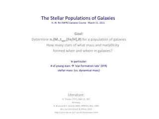
The Stellar Populations of Galaxies H.-W. Rix IMPRS Galaxies Course March 11, 2011. Goal: Determine n * (M * , t age ,[Fe /H], R ) for a population of galaxies How many stars of what mass and metallicity formed when and where in galaxies? In particular:

E N D
The Stellar Populations of GalaxiesH.-W. Rix IMPRS Galaxies Course March 11, 2011 Goal: Determine n*(M*,tage,[Fe/H],R)for a population of galaxies How many stars of what mass and metallicity formed when and where in galaxies? In particular: # of young stars ‘star formation rate’ (SFR) stellar mass (vs. dynamical mass) Literature: B. Tinsley, 1972, A&A 20, 383 Worthey G. Bruzual & S. Charlot 2003, MNRAS, 344, 1000 Mo, van den Bosch & White 2010 http://astro.dur.ac.uk/~rjsmith/stellarpops.html
Physical vs. observable properties of stars • Stellar structure: Lbolom = f(M,tage,[Fe/H]), Teff = f(M,tage,[Fe/H]) • Most stars spend most of their time on the main sequence (MS), • stars <0.9 Msun have MS-lifetimes >tHubble • M=10 Msun are short-lived: <108 years ~ 1 torbit • Only massive stars are hot enough to produce HI – ionizing radiation • LMS(M)~M3 massive stars dominate the luminosity (see ‘initial mass function’) • Model predictions are given as ‘tracks’ (fate of individual stars) , or as isochrones, i.e. population snapshots at a given time (Padova, Geneva, Yale, etc… isochrones) ‘isochrones’: where stars of different mass live at a given age Teff or ‘color’ ‘tracks’ of individual stars in the L-Teff plane as a function of time
Information from Stellar Spectra Stellar spectra reflect: • spectral type (OBAFGKM) • effective temperature Teff • chemical (surface) abundance • [Fe/H] + much more e.g [a/Fe] • absorption line strengths depend on Teff and [Fe/H] modelling • surface gravity, log g • Line width (line broadening) • yields: size at a given mass • dwarf - giant distinction for GKM stars • no easy ‘age’-parameter • Except e.g. t<tMS theoretical modelling of high resolution spectra metal poor metal rich
Resolved Single Stellar Populations(photometry only) • ‘Single stellar populations’ (SSP) • tage, [Fe/H], [a,Fe], identical for all stars • open and (many) globular clusters are SSP • Isochrone fitting • transform Teff (filter) colors • distance from e.g. ‘horizontal branch’ • Get metallicity from giant branch color • only for t>1Gyr • no need for spectra • get age from MS turn-off • Ages only from population properties! • N.B. some degeneracies
The Initial Mass Function and ‘Single Stellar populations’ • Consider an ensemble of stars born in a molecular cloud (single stellar population) • The distribution of their individual masses can be described piecewise by power-laws N(M) ∝ M-αdM (e.g. Kroupa 2001) • N(M) ∝ M-2.35dM for M>Msun (Salpeter 1953) • much of integrated stellar mass near 1Msun • Massive stars dominate MS luminosity, because LMS ~ M3 • For young populations (<300 Myrs) • upper MS stars dominate integrated Lbol • For old populations (>2Gyrs) • red giants dominate integrated Lbol Bulk of mass integral
Resolved Composite Stellar Populations(photometry only) Synthetic CMD from D. Weisz • ‘Composite stellar populations’ • tage, [Fe/H], [a,Fe] vary • stars have (essentially) the same distance • Examples: nearby galaxies • Full CMD (Hess diagram) fitting • Both locus and number of stars in CMD matter • Forward fitting or deconvolution • Result: estimate of f(tage,[Fe/H]) Hess diagram CMDs for different parts of LMC LMC: Zaritsky & Harris 2004-2009
Constructing the Star-Formation History (SFH) for Resolved Composite Stellar Populations • Convert observables to f(tage,[Fe/H]) • E.g. Leo A (Gallart et al 2007) • LMC (e.g. Harrison & Zaritsky) • Issues • Not all starlight ‘gets out’ • Dust extinction dims and reddens • Star light excites interstellar • Age resolution logarithmic, i.e. 9Gyrs =11Gyrs • Basic Lessons (from ‘nearby’ galaxies, < 3Mpc) • All galaxies are composite populations • Different (morphological) types of galaxies have very different SFH • Some mostly old stars (tage >5Gyrs) • Some have formed stars for t~tHubble • younger stars higher [Fe/H] • Multiple generations of stars self-enrichment Metal poor Metal rich metal rich metal poor
‘Integrated’ Stellar Populations • of the >1010 galaxies in the observable universe, only 10-100 are ‘resolved’ • What can we say about f(tage,[Fe/H]), SFR, M*,total for the unresolved galaxies? • galaxies 5-100Mpc stars are unresolved but stellar body well resolved • z>0.1 means that we also have to average over large parts of the galaxy • Observables: • colors, or ‘many colors’, i.e the ‘spectral energy distribution’ (SED) (R=5 spectrum) • Spectra (R=2000) integrated over the flux from ‘many’ stars • covering a small part (e.g. the center) of the galaxy, or the entire stellar body
Describing Integrated Stellar Populations by ColorsIntegrating (averaging) destroys information • Straightforward: predict • assume SFH, f(tage,[Fe/H],IMF) flux, colors • Isochrones for that age and [Fe/H] • IMF, distribution of stellar masses • Translate Lbol.Teff to ‘colors’ • post-giant branch phases tricky • Dust reddening must be included • Impossible: invert • invert observed colors to get f(tage,[Fe/H],IMF) • Doable: constrain ‘suitable quantities’ • Infer approximate ( M/L )* • Check for young, unobscured stars (UV flux) • Test which set of SFH is consistent with data • NB: different colors strongly correlate • ‘real’ galaxies form a 1-2D sequence in color space
Stellar Population Synthesis Modellinge.g. Bruzual & Charlot 2003; da Cunha 2008 5) SED ‘integrated spectrum’: 3) ‘isochrones’: what’s Teff and L =f(M*,age) 1) Assume star formation history (SFH ) (M*,[Fe/H]) + 2) ‘IMF’: how many stars of what mass SFR [Mo/yr] time [Gyrs] 4) Spectral library: What does the spectrum look like = f(Teff,logg, [Fe/H] 6) Band-pass integration: Integrate spectrum over bandpass to get colors N(M)dM log(M/Mo)
The Integrated SED’s of Simple Stellar Populations • Populations fade as they age • ionizing flux is only produced for t<20 Myrs • Fading by • X 105 at 3000A from 10 Myrs to 10Gyrs • UV flux is only produce for 0.2Gyrs • X 100 at 5000A from 0.1Gyrs to 10Gyrs • X 6at 1.5mm from 1Gyr to 10Gyrs • populations ‘redden’ as they age • Higher ‘metallicity’ and dust also ‘redden’ • Spectral features • There are ‘breaks’ in the spectrum: • Ly break 912A • Balmer break & 4000A break • 1.6mm ‘bump’ • Hydrogen vs metal lines: >1Gyr or <1Gyr • >1 Gyr: all signatures become sublte • Integrated spectra of young populations also have emission lines tstars = [Gyrs]
SED Modelling: A worked example or z>1 galaxiescourtesy E. da Cunha Data: • Fluxes & errors in ~20 bands • taken from different instruments • averaged over the entire galaxy What you fit for: • redshift (‘photometric redshift) • Stars formation rate (t<20Myrs) • stellar mass • Fraction of light absorbed by dust • (dust spectrum) • Also: • ‘marginalize’ over possible SFHs • convert to physical quanities using the luminosity distance Best-fit model spectrum Data points Un-extincted model spectrum Star-Formation Rate Dust extinction Stellar mass
Application I: Estimating ‘Star Formation Rates’ Integrated spectrum of a ,blue’, star-forming galaxy • “SFR” = M*(tage <Dt)/Dt • Dt= 10 – 200 Myrs • NB: SFR may vary within Dt • SFR estimates are all based on counting either • Ionizing photons, often reflected in Ha • UV photons (only from short-lived stars) • Dust heated by UV photons • Fraction of absorbed UV photons varies from 10% to nearly 100% • Higher extinction in more massive (metal rich) galaxies and at high SFR • SFR estimates depend entirely on IMF • effects from M*>5Mo • those stars contribute negligibly to Mtot Integrated spectrum of a red ‘passive’ galaxy (?) Ln(inUV)~const for very young pos.s (e.g. Kennicutt 98)
Getting Stellar Mass-to-light Ratios from spectra/colors Bell & de Jong 2001Kauffmann et al 2004 • Define ‘line indices; (e.g. D4000), EW Hd to characterize the spectrum • Different observed spectra fall onto a 2 dimensional sequence (blue to red) • To get a first guess at the stellar mass-to-light ratio, it is enough to measure one optical color, e.g. g-r • Bell & de Jong 2001 SSP Cont. SFR Obs. Z=0.1 SDSS galaxies
What can we learn from such modeling?Applications from SDSS to present epoch (z~0.05) galaxies • The distribution of stellar galaxy masses • Take large sample of galaxies • Determine M*(SED) for each galaxy • Correct for V/Vmax for any random star in the present day universe, what is the chance that it lives in a galaxy whose total stellar mass is M* most stars live in galaxies with 1010 – 2x10¹¹Mo • How rapidly are galaxies making new stars now? • Calculate ‘specific star formation rate’ (SSFR) SFR(now)/<SFR>(past) • Galaxies with M*> 2x10¹¹ hardly form new stars
What do we learn from such modeling? • Try to invert SFH of galaxies from present-day spectra (Heavens et al 2004) • Assume SFR = A x exp( - t/tscale) for all galaxies • tscale large constant star formation rate • Determine A, tscale for each galaxy SFH • Proper average over all galaxies in sample volume • Global (volume averaged) SFH has dropped by ~5-10 since z=1 • Lower mass galaxies have a more prolonged SFH Heavens et al 2004
Population diagnostics in ‘old’ (>2 Gyrs) populations • Nowadays, the majority of stars live in galaxies with ‘old’ populations • massive ‘early-type’ galaxies • Use of ‘line indices’ • Lick indices – EW measurements • focus on interesting parts of spectra • Age and metallicity are nearly completely degenerate! • Balmer lines as age diagnostics • Massive galaxies have higher Mg/Fe ratios ([a/Fe]) than the Sun • Enhanced [a/Fe]: SN Ia – deficient (i.e. rapid) chemical enrichment • Multiple generations of stars formed rapidly (?) Mod el EW predictions vs. Observed ellipticals in the Coma cluster
Stellar populations: Summary • For resolved populations one can reconstruct f(tage,[Fe/H]) from CMD’s • need good distances • Need CMDs that reach the MS-turn-off of the oldest population • Integrated colors or spectra • Cannot be robustly inverted to yield f(tage,[Fe/H]) • (M/L)* can be robustly (better than x2) determined, for assumed IMF • Star formation rates (to ~ x2) can be determined, from Ha, UV, thermal IR • SED/spectral modelling covering a wide wavelength range is best approach. • SDSS spectra and colors have given us a clear picture of the present-day galaxy population in physical units, M*, SFR. • More massive galaxies have a larger fraction of old stars • Massive galaxies (5x10¹⁰) barely form new stars