Download

1 / 15

E N D
Concepts of Cost • Given a firm’s production technology, managers must decide ‘how’ to produce. As the inputs can be combined in various ways to yield the same amount of output, we are interested in how the ‘optimal’ (cost-minimising) combination of inputs is chosen, given the factor prices. • There are differences with the concept of cost between the economists and the accountants, who are concerned with the firm’s financial statements. • Accounting cost includes depreciation expenses for capital equipment, which are determined on the basis of the allowable tax treatment according to the Taxation Rules of the country. • Economists are concerned with what cost is expected to be in the future, and with how the firm might be able to rearrange its resources to lower its cost and improve profitability. Thus, they are concerned with “opportunity cost”.
Cost in the Short Run • Total cost of production has two components: • Fixed cost, FC, which is borne by the firm whatever level of output it produces, • Variable cost, VC, which varies with the level of output. • Depending upon the circumstances, FC may include expenditures for plant maintenance, insurance, and perhaps a minimal no. of employees – this cost remains same no matter how much the firm produces. • Fixed cost must be paid even if there is no output. • Variable cost includes expenditures for wages, salaries, and raw materials – this cost increases as output increases.
Cost in the Short Run Marginal cost (MC) • It is the increase in cost that results from producing one extra unit of output. Because FC does not change as the firm’s level of output changes, MC is just the increase in variable cost that results from an extra unit of output. • MC tells us how much it will cost to expand the firm’s output by one unit.
Cost in the Short Run Average cost (AC) • Average cost is the cost per unit of output. Average Total cost (ATC) is the firm’s total cost divided by its level of output. ATC has two components: • Average Fixed Cost – AFC is the fixed cost divided by the level of output • Average Variable Cost – AVC is variable cost divided by the level of output
Variable and total costs increase with output. The rate at which these costs increase depends on the nature of the production process, and in particular on the extent to which production involves diminishing returns to variable factors. Shapes of Cost Curves in the Short Run Cost Total Cost Total Variable Cost Total Fixed Cost Quantity
Shapes of Cost Curves in the Short Run AFC AFC AP Quantity Average Product AC Average Cost Quantity
Whenever marginal cost lies below average cost, the AVC curve falls. Whenever MC lies above average cost, the AVC curve rises. And when average cost is at a minimum, MC curve equals average cost. Relation between Cost Curves in the Short Run MC, AVC Average Variable Cost Marginal Cost Quantity
Since the difference between ATC and AVC is the AFC, which continuously declines as output increases, the gap between ATC and AVC curves narrows further; however AVC & ATC curves never meet as AFC never becomes zero. The MC curve passes through the minimum points of both ATC and AVC curves Relation between Cost Curves in the Short Run MC, AVC ATC Average Total Cost Marginal Cost Average Variable Cost Quantity
Relation between Cost Curves in the Short Run • Knowledge of short-run costs is particularly important for firms that operate in an environment in which demand conditions fluctuate considerably. If the firm is currently producing at a level of output at which MC is sharply increasing, and demand may increase in future, the firm might consider expanding its production capacity to avoid higher costs.
Long-run Average Cost • The most important determinant of the shape of the long-run average and marginal cost curves is whether there are increasing, constant, or decreasing returns to scale. • If the firm’s production process exhibits constant returns to scale at all levels of output, then a doubling of inputs leads to a doubling of output. Because input prices remain unchanged as output increases, the average cost of production must be same for all levels of output. • If the firm’s production process exhibits increasing returns to scale at all levels of output, then a doubling of inputs leads to more than doubling of output. Then the average cost of production falls with output because a doubling of costs is associated with more than two-fold increase in output.
Long-run Average Cost • In the long-run, most firms’ production technology first exhibit increasing returns to scale, then constant returns to scale, and eventually decreasing returns to scale.
Shape of Long-run Average Cost • Economists think that the LRAC is U-shaped mainly because of: • Downward falling section is due to Economies of Scale • Flat section – mainly due to constant returns to scale • Upward rising section of LRAC is due to Diseconomies of Scale
Long-run Marginal Cost • LRMC measures the change in long-run total costs as output is increased incrementally. LMC lies below the LRAC curve when long-run average cost is falling; and above the LRAC curve when long-run average cost is increasing. • The two curves intersect where the LRAC curve achieves its minimum.
Long-run Marginal Cost • Q* is the optimal plant size/ scale. At this level of output, SRAC is also at its minimum, and hence is said to operate at the optimum level of output. Any level of output below or above would exhibit below capacity or above capacity.