Download
1 / 43
460 likes | 693 Views
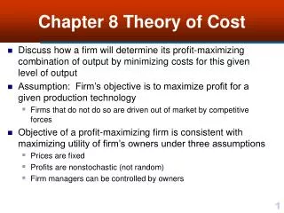
Chapter 8 Theory of Cost. Discuss how a firm will determine its profit-maximizing combination of output by minimizing costs for this given level of output Assumption: Firm’s objective is to maximize profit for a given production technology

E N D
Chapter 8 Theory of Cost • Discuss how a firm will determine its profit-maximizing combination of output by minimizing costs for this given level of output • Assumption: Firm’s objective is to maximize profit for a given production technology • Firms that do not do so are driven out of market by competitive forces • Objective of a profit-maximizing firm is consistent with maximizing utility of firm’s owners under three assumptions • Prices are fixed • Profits are nonstochastic (not random) • Firm managers can be controlled by owners
Introduction • Profit maximizing requires deciding • How much output to produce • How much of various inputs to use in producing this output • Constraints on maximizing profit are • Technological relationship between output and inputs (characterized by a production function) • Prices of inputs • Prices of outputs • Determining profit-maximizing combination of inputs and outputs may be decomposed into two parts • Firm will minimize cost for a given level of output • Firm will determine its profit-maximizing output
Introduction • Aim in this chapter is to • Develop family of cost curves in both short and long run • Cost curves incorporate technology used for producing an output with given input prices • Two general classifications of costs are • In terms of who owns input for which cost is incurred • Whether cost is associated with a fixed or variable input • We investigate family of long-run cost curves in terms of returns to scale • We derive short-run cost curves by fixing one of the inputs • We discuss shifts in cost curves, resulting from a change in input prices, and development of new technologies
Explicit And Implicit Costs • Firm’s cost of production involves • Inputs firm purchases in market • Such as additional labor or additional capital equipment • Inputs firm already owns • Such as owner’s labor, land, or equipment • Explicit (or expenditure) costs • Costs of employing additional inputs not owned by firm • Includes all cash or out-of-pocket expenses incurred in production • Accounting cost for purchased inputs whether they are fixed or variable
Explicit And Implicit Costs • Implicit costs (also called nonexpenditure, imputed, or entrepreneurial costs) • Costs charged to inputs that are owned by firm • An opportunity cost of using an input in production of a commodity • Loss in benefits that could be obtained by using these inputs in another activity • Owners of firm also have an implicit cost associated with time devoted to a particular production activity • Total cost (TC) of a particular production activity • Sum of explicit plus implicit costs
Fixed And Variable Costs • Costs can also be classified according to whether they are • Fixed • Costs that do not vary with changes in output • Variable • Costs associated with variable inputs and do vary with output • Explicit and implicit costs may contain both fixed and variable costs • Total cost (TC) is sum of fixed and variable costs • Figure 8.1 illustrates how total cost may be decomposed
Figure 8.1 The makeup of total cost in the short and long run
Profits • Define profits as • Normal • Minimum total return to the inputs necessary to keep a firm in a given production activity • Also called necessary, ordinary, or opportunity-cost profit • Equals implicit cost • Pure • Total return above total cost • Also called economic profit • In short run, possibility of earning a pure profit exists but firms will only earn a normal profit in long run • In long run, firms have ability to enter or exit an industry • Will not operate at a loss or earn a pure profit
Cost-Minimizing Input Choice • We investigate cost-minimizing approach for a given level of output under two assumptions • Two inputs are used in production • Perfectly competitive input markets exist • Firm takes input prices as fixed • Supply curves are horizontal and perfectly elastic
Long-run Costs: Isocost • Within relevant region of isoquant map, we determine least-cost combination of inputs for a given level of output by considering cost of variable inputs • Cost can be represented by isocost curves • Analogous to budget lines in consumer theory
Long-run Costs: Isocost • Associated isocost equation is • TC = wL + vK • w is wage rate of labor • v is per-unit input price of capital • For a movement along an isocost curve, firm’s cost of production remains fixed • Solving isocost equation for K • K = -w/vL + TC/v • Results in a linear equation with TC/v as the capital (K), intercept • -w/r as slope • Illustrated in Figure 8.2
Long-run Costs: Isocost • For a given fixed amount of TC, intercept TC/v is amount of capital (K) that can be purchased if no labor (L) is purchased • TC/w is amount of labor that can be hired if no capital is purchased • Slope indicates market rate at which labor can be purchased in place of capital, holding TC constant • An increase in TC causes a parallel upward shift in isocost curve
Least-Cost Combination of Inputs • Lowest TC is called long-run total cost (LTC) • LTC = min(wL + vK), s.t.q° = (K, L) • Where (wL + vK) is isocost equation representing total cost of inputs • Profit-maximizing firm is interested in minimizing this TC • Called allocative efficiency • Results in determination of least-cost combination of inputs for each possible level of output • Firm can maximize profits by selecting its optimal level of output
Least-Cost Combination of Inputs • Isoquant represents given level of output, q° • Objective of firm is to shift to a lower isocost curve • Reduce costs until least-cost combination of inputs is obtained for output q° • At point B firm can no longer reduce TC by moving along isoquant • At point B, isocost and isoquant curves are tangent • In least-cost combination of inputs, price per marginal product of each input must be equivalent • When deciding on amount of inputs to hire, a firm will attempt to equate price per marginal product for all inputs it purchases • Price of an input per additional increase in output is the same for all inputs
Expansion Path • Locus of points where isoquant curve and isocost line are tangent is called expansion path • See Figure 8.3 • Some level of output can still be produced with zero capital • Generally, an expansion path has a positive slope • An increase in LTC, required for producing a higher level of output, results in both inputs increasing
Long-Run Total Cost • Given expansion path in Figure 8.3, can construct LTC curve • By plotting output levels with corresponding minimal level of long-run cost (Figure 8.4) • LTC provides lowest cost necessary for obtaining a given level of output • Every pointon LTC curve corresponds to a tangency between an isoquant and an isocost line (Figure 8.3) • Slope of LTC curve is LMC • LMC = ∂LTC/∂q • Long-run average cost (LAC) • LAC = LTC/q
Returns to Scale • Returns to scale can be directly related to long-run cost curves • A cost curve may exhibit increasing, decreasing, and/or constant returns to scale • Increasing returns to scale (also called economies of scale) is where LAC is declining • ∂LAC/∂q < 0 • Increases in total cost are proportionally smaller than an increase in output • Implies that inputs less than double for a doubling of output • Corresponds to LTC also less than doubling
Returns to Scale • Decreasing returns to scale (also called diseconomies of scale) is where LAC is increasing • ∂LAC/∂q > 0 • Increases in total cost are proportionally larger than an increase in output • Implies that inputs more than double for a doubling of output • Corresponds to LTC more than doubling for a doubling of output • Constant returns to scale (also called constant economies of scale) corresponds to where ∂LAC/∂q = 0 • Long-run average cost does not change for a given change in output • If LTC curve is linear, then constant returns to scale exists for all levels of output • Illustrated in Figure 8.6
Figure 8.6 Linear long-run total cost curve representing constant returns to scale
Average and Marginal Cost Relationship • Relationship between average and marginal units also applies to average and marginal costs • When a marginal unit is below average, average is falling • If LMC is below LAC, so average is falling • At minimum point of LAC, LMC is equal to LAC • LMC crosses LAC at minimum point of LAC • If an average unit is neither rising nor falling, marginal unit is equal to it
Short-run Costs: Total Costs • STC, including both explicit and implicit costs, is defined as short-run total variable cost (STVC) plus total fixed cost (TFC) • Assuming that capital is fixed at K° in short run • STC(K°) = STVC(K°) + TFC(K°) = min(wL + vk°) • (wL + vk°) is isocost equation • STVC(K°) = wL* and TFC(K°) = vk° • L* denotes level of labor that minimizes costs for a given level of output • TFC represents explicit and implicit costs that do not vary with output
Short-run Costs: Total Costs • Even if firm were to produce nothing, in short run it must still pay TFC • TFC is a horizontal line, showing that at all output levels, TFC remains the same • See Figure 8.8 • STVC represents explicit and implicit costs that vary directly with output • STVC at first increases at a decreasing rate and then increases at an increasing rate • Due to Law of Diminishing Marginal Returns
Average Costs • Short-run costs can be further classified as • Short-run average total cost (SATC) • Short-run average variable cost (SATC) • Average fixed cost (AFC) • Derive all of these average costs by dividing short-run total cost by output • For a fixed level of capital K° • SATC(K°) = STC(K°)/q = SAVC(K°) + AFC(K°) • Where SAVC(K°) = STVC(K°)/q and AFC(K°) = TFC(K°)/q • AFC is continually declining as output increases • As output tends toward zero (infinity), AFC approaches infinity (zero) • SATC and SAVC never intersect • Approach each other as output increases
Marginal Cost • Short-run marginal cost (SMC) for a fixed level of capital K° is defined as • STC and STVC are vertically parallel • Due to Law of Diminishing Marginal Returns, SMC may at first decline • Reach a minimum at point of inflection of STC and STVC • Then rise with increases in output
Isoquant Map and STC • Can construct short-run cost curves by fixing level of one input in isoquant map and varying level of output (Figure 8.11) • For example, at level of output q1, with capital fixed at K°, isocost curve associated with STC(K°)1 represents minimum cost of producing q1 with fixed level of capital K° • In long run, allowing capital to vary further decreases this short-run minimum cost • Represented by isocost line LTC1 • Because minimizing costs in short run is a constrained version of long-run minimization, STC cannot be less than LTC • STC will be equal to LTC only where level of fixed inputs is least-cost amount of input for producing given level of output • In Figure 8.11, this corresponds to output level q2
Figure 8.11 Short-run total cost as a constrained minimization of long-run total cost
Relationships Between Short- And Long-run Cost Curves • In general, there are an infinite number of short-run total cost curves • One for every conceivable level of fixed input • As level of capital is varied, a new STC curve is traced out and is tangent to LTC at that level of fixed capital that is the long-run optimal input usage • (Figure 8.12) • STC curves for alternative levels of fixed input capital completely cover top of LTC curve and will not dip below it • STC is a constrained cost-minimization version of LTC, constrained by some given level of fixed input capital • LTC is not constrained by this level of fixed capital • Will never result in a higher cost than STC for a given level of output
Figure 8.12 Long-run total cost curve derived from the envelope of the short-run total cost curves
Relationships Between Short- And Long-run Cost Curves • We derive long-run average cost (LAC) and long-run marginal cost (LMC) curves from LTC curve (Figure 8.13) • Where STC is tangent to LTC, SATC is also tangent to LAC • Because averages are totals divided by given level of output • Tangency by definition implies that slopes of STC and LTC are equal at a point of tangency • SATC curves envelop top of LAC curve • SATC cannot be less than LAC for a given level of output • SATC curve cannot dip below LAC curve • LMC curve will be horizontal and equal to LAC if cost curves exhibit constant returns to scale (Figure 8.14) • Minimum points of SATC are tangent to horizontal LAC curve
Figure 8.13 Long-run average cost and long-run marginal cost curves with economies …
Figure 8.14 Short-run total cost and long-run total cost curves for a firm facing constant …
Input Price Change • A change in price of an input will tilt firm’s isocost line • For example, in long run, an increase in wage rates results in a firm producing any output level with relatively more capital and relatively less labor • Elasticity of substitution results in entire expansion path of firm rotating toward capital axis • Illustrated in Figure 8.15 • Long-run total cost curve will tilt to left
Figure 8.15 Change in an input price and resulting shift in the expansion path and …
Input Price Change • In short run, an increase in price of a variable input will tilt short-run total variable cost and total cost curves • As indicated in Figure 8.16, SAVC, SATC, and SMC curves will also shift • However, an increase in price of a fixed input does not shift STVC, SAVC, and SMC curves (Figure 8.17) • Curves are not dependent on price of fixed input • Only SATC curve shifts
Figure 8.16 Change in a variable input price and resulting shifts …
Figure 8.17 Change in a fixed input price and resulting shifts in the short-run …
New Technologies • Development of a new technology that alters a firm’s production function • Results in isoquants shifting toward origin • Causes cost curves to shift downward • See Figure 8.18
Figure 8.18 Change in technology causing a shift in the short-run …
Positive Feedback • Small chance events in history of an industry or technology can tilt competitive balance toward a firm • May allow firm to increase output and experience increasing returns to scale