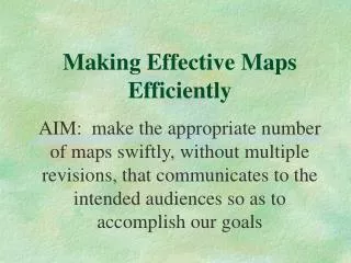
Making Effective Maps Efficiently

1. Making Effective MapsEfficiently AIM: make the appropriate number of maps swiftly, without multiple revisions, that communicates to the intended audiences so as to accomplish our goals

2. ArcView’s power paradoxically can limit efficient map production: • offers many options • doesn’t help people make design choices • as computer-based tool, encourages managers to expect easy, multiple revisions • thus mapmakers rarely take time to consider communication effectiveness of their maps, reducing chances of success

3. Decisions to Get Started . who your audience(s) is (are) . what your message(s) will be . where the map will be used (oral presentation; report; newspaper/TV) . what data to map . how many maps are needed to present the message(s) to audience(s) in what locations

4. Who Your Audience is • your immediate superior • fellow program staff • other programs’ staff • senior managers (Management Team, etc.) • legislature/Governor • stakeholders (industry, environmentalists…) • general public (attentive; non-attentive)

5. Why Considering Audiences is Important Effective communication depends upon: (1) understanding what information your audience wants about the topic (2) understanding how your audience might interpret the information you want to give them (3) incorporating (1) and (2) into map design

6. What the Message Will Be • What the agency knows • What the agency does/will do • What reactions the audience might take • Reasons for agency/audience reaction

7. Where the Map Will Be Used • Affects the complexity of the message that can be conveyed. • Affects the ability to offer supplementary information. (e.g. text, graphics) • Affects text and symbol choices. • Affects color choices (beware of designing in color but printing in black & white)

8. What Data to Map • The most current data • The most accurate data • Data that pertains to area of interest • Data that is readily understood by intended audience.

9. How Many Maps are Needed • Complexmaps, especially those with more than one message, are not easily understood. • If you make your audiences work too hard to interpret your map, they may be distracted from your message

10. Audience-Message-Venue-Data Affects: • Map Type, Display Type • Data Type • Symbolization • Graphic Hierarchy • Geographic Frame of Reference • Color

11. Map Types Choose the most appropriate one based on your message, data, audience and venue

12. Standard

13. Images

14. Choropleth Unique Value

15. Choropleth Graduated Color

16. Graduated Symbol

17. Chart

18. Dot Density

19. 3-D

20. Statistical Analysis Result of a T-test performed to identify areas of significant change in deer harvest.

21. DATA TYPES The most important factor in determining map type and symbols

22. Qualitative Data Differences in Kind Point

23. Polygon

24. Line

25. Quantitative Data Differences in amounts and measures . Point Data - Discrete vs. Continuous e.g. chemical releases at a site (discrete) e.g. rainfall (continuous) . Polygon Data - Absolute vs. Ratio e.g. number of persons (absolute) e.g. population density (ratio) . Line Data e.g. flow lines, thickness of line

26. Point Data Discrete vs. Continuous Discrete Continuous

27. Polygon Data – absolute & ratio Population Pop Den Incorrect Correct

28. Population - 1990 Incorrect

29. Population Density Correct

30. Population Correct

31. Line Data

32. SYMBOLIZATION The key to communicating to your audience

33. Legends Qualitative Data Use professional standards whenever possible Make symbols as intuitive as possible

34. Quantitative Data • Natural Breaks (default) • Quantile • Equal Area • Equal Interval • Standard Deviation

35. Natural Breaks . ArcView’s default classification method. .Identifies break points by looking for groupings and patterns inherent in the data. Extreme values are obvious.

36. Natural Breaks - example

37. Quantile . Each class is assigned the same number of features. . It doesn’t matter if features on either side of a class boundary have almost the same values. . Best suited for a data set that does not have a large number of features with similar values.

38. Quantile - example

39. Equal Area . Classifies polygon features by finding breakpoints in the attribute values so that the total area of the polygons in each class is approximately the same. . Polygons with the largest values tend to hide variation in population between geographically smaller areas.

40. Equal Area - example

41. Equal Interval . The range of attribute values is divided into equal sized sub-ranges. . Useful when you want to emphasize the amount of an attribute value relative to another value. (e.g. If you want to show that a municipality is part of a group of municipalities that make up the bottom 20% for population density). . Not good if you want to reveal subtle differences between features with similar values.

42. Equal Interval - example

43. Standard Deviation . Shows you the extent to which an attribute’s values differ from the mean of all the values. . ArcView first finds the mean value and then places the class breaks above and below the mean at 1, .5, or .25 standard deviations. . ArcView will aggregate any values beyond three standard deviations from the mean into two classes: ‘>3 Std Dev’ and ‘<3 Std Dev’.

44. Standard Deviation - example

45. Loading Legend Symbols

46. Loading legend symbols continued

47. Loading and Saving a Legend

48. Loading and Saving a Legend continued

49. Loading and Saving a Legend continued

50. Rotating Point symbols can be rotated to symbolize additional information about features. e.g. wind direction