Download
1 / 21
210 likes | 303 Views
Explore the issue of sampling error in psychological research, learn about null-hypothesis significance tests, and how to interpret research results accurately.

E N D
The problem of sampling error in psychological research • We previously noted that sampling error is problematic in psychological research because differences observed between experimental conditions could be due to real differences or sampling error.
Example of the problem • Example: We want to know whether psychotherapy increases people’s psychological well-being. The average well-being of Chicagoans is 3.00 (SD = 1). We give a randomly sampled group of 25 Chicagoans therapy. Months later, we measure their well-being. The average well-being in this sample is 3.50.
Big Question • Is the .50 difference between the therapy group and Chicagoans in general a result of therapy or an “accident” of sampling error? • Note: There are two hypotheses implied in this question: • The sample comes from a population in which the mean is 3.00, and the difference we observed is due to sampling error. (Often called the “null hypothesis.”) • The sample does not come from a population in which the mean is 3.00. The difference is due to therapy. (Often called the “research hypothesis” or “alternative hypothesis.”)
How can we determine which of these hypotheses is most likely to be true? • The most popular tools for answering this kind of question are called Null-Hypothesis Significance Tests (NHSTs). • Significance tests are a broad set of quantitative techniques for evaluating the probability of observing the data under the assumption that the null hypothesis is true. This information is used to make a binary (yes/no) decision about whether the null hypothesis is a viable explanation for the study results.
Basic Logic of NHST • If we assume the null hypothesis is true (e.g., the difference between our sample mean and the population mean is due to sampling error), then we can generate a sampling distribution that characterizes the the distribution of sample means we might expect to observe. • That is, if we make certain assumptions about the population (e.g., mu = 3) and the sampling process (e.g., random sampling, N = 25), we can determine (a) the expected sample mean and (b) the expected difference between an observed sample mean and the population mean when a sampling error is made. • If the probability of observing our sample mean under these assumptions is “small,” we reject the null hypothesis. • If the probability of observing our sample mean under these assumptions is “large,” we accept the null hypothesis.
Sampling distribution for the mean Mean is 3.00 SD (SE) = 0.20 [1/sqrt(25) = .20]
Recall that we can find the proportion of sample means that fall between specific values. We can interpret these as probabilities in the relative frequency sense of the term. 34% 14% 2 %
*** We can use these probabilities to determine how likely it is that we will observe a range of sample means based on sampling error alone. Note: This is the same logic we used when we constructed confidence intervals in the last lecture. *** • In our example, the probability of observing a sample mean between 2.8 and 3.2 is 68%. • The probability of observing a sample mean equal to or greater than 3.5 is approximately 1%.
How NHSTs work • Is 1% a “small” probability? • Because the distribution of sample means is continuous, we must create an arbitrary point along this continuum for denoting what is “small” and what is “large.” • By convention, if the probability of observing the sample mean is less than 5%, researchers reject the null hypothesis.
The probability of observing a mean of 3.5 or higher is less than 5%. M = 3.5
Rules of the NHST Game • This probability value is often called a p-value or p. • When p < .05, a result is said to be “statistically significant” • In short, when a result is statistically significant (p < .05), we conclude that the difference we observed was unlikely to be due to sampling error alone. We “reject the null hypothesis.” • If the statistic is not statistically significant (p > .05), we conclude that sampling error is a plausible interpretation of the results. We “fail to reject the null hypothesis.”
It is important to keep in mind that NHSTs were developed for the purpose of making yes/no decisions about the null hypothesis. • As a consequence, the null is either accepted or rejected on the basis of the p-value. • For logical reasons, some people are uneasy “accepting the null hypothesis” when p > .05, and prefer to say that they “failed to reject the null hypothesis” instead. • This seems unnecessarily cumbersome to me, and divorces the technique from its original decision-making purpose. • In this class, please feel free to use whichever phrase seems most sensible to you.
Points of Interest • The example we explored previously was an example of what is called a z-test of a sample mean. • Significance tests have been developed for a number of statistics • difference between two group means: t-test • difference between two or more group means: ANOVA • differences between proportions: chi-square
We’ll discuss some common problems and misinterpretations of p-values and NHSTs in two weeks, but, for now, there are a few of things that you should bear in mind in the meantime: • (1) The term “significant” does not mean important, substantial, or worthwhile.
(2) The null and alternative hypotheses are often constructed to be mutually exclusive. If one is true, the other must be false. • As a consequence, • When you reject the null hypothesis, you accept the alternative. • When you accept the null hypothesis, you reject the alternative. • This may seem tricky because NHSTs do not test the research hypothesis per se. Formally, only the null hypothesis is tested. • In addition, the logical problems discussed previously are relevant here.
(3) Because NHSTs are often used to make a yes/no decision about whether the null hypothesis is a viable explanation, mistakes can be made.
Inferential Errors and NHST Real World Null is true Null is false Correct decision Type II error Null is true Conclusion of the test Correct decision Null is false Type I error
Errors in Inference using NHST • Type I error: Your test is significant (p < .05), so you reject the null hypothesis, but the null hypothesis is actually true. • Type II error: Your test is not significant (p > .05), you don’t reject the null hypothesis, but you should have because it is false.
Errors in Inference using NHST • The probability of making a Type I error is determined by the experimenter. Often called the alpha value. Usually set to 5%. • The probability of making a Type II error is determined by the experimenter. Often called the beta value. Usually ignored by researchers.
Errors in Inference using NHST • The converse of Type II error is called Power: the probability of rejecting the null hypothesis when it is false—a correct decision. 1- beta • Power is strongly influenced by sample size. With larger N, more likely to reject null if it is false. • Note: N does not influence the likelihood of making a correct decision if the null hypothesis is true (i.e, not rejecting null). This probability is always equal to 1-alpha, regardless of sample size.