Regression in R

1. Regression in R Stacia DeSantis March 23, 2011 Computing for Research I

2. Introduction • For linear regression, R uses 2 functions. • Could use built in function “lm” • Could use the generalized linear model (GLM) framework • Built in function called “glm” • A linear regression is a type of GLM. • Recall, GLM contains: • A probability distribution from the exponential family • A linear predictor • A link function g

3. Linear Regression • To implement linear regression using glm function, we must know: • The exponential family distribution assumed is Normal that is (Y|X) ~ Normal(μ,σ2) • The linear predictor is η = Xβ • The link function is the identity link, E(Y|X) = μ = Xβ • must know: • These distribution, linear predictor and link function will be specified in the glm function call

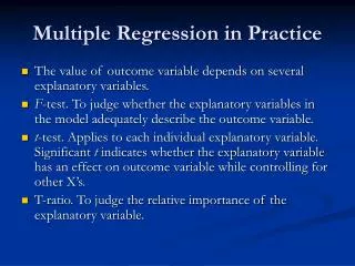
4. Data dependent Variable (Y) Independent Variable (X) RECALL, Simple linear regression describes the linear relationship between a predictor variable, plotted on the x-axis, and a response variable, plotted on the y-axis

5. ε Y ε X

6. Y 1.0 X

7. Fitting data to a linear model intercept slope residuals

8. Data Mean Height versus Age in Months

9. Read Data into R age <- c(18,19,20,21,22,23,24,25,26,27,28,29) height <- c(76.1,77,78.1,78.2,78.8,79.7,79.9,81.1,81.2,81.8,81.8,83.5) dat <- as.data.frame(cbind(age,height)) dat dim(dat) is.data.frame(dat) names(dat)

10. LM function in brief • http://stat.ethz.ch/R-manual/R-patched/library/stats/html/lm.html • lm(formula, data, subset, weights, na.action, method = "qr", model = TRUE, x = FALSE, y = FALSE, qr = TRUE, singular.ok = TRUE, contrasts = NULL, offset, ...) • reg1 <- lm(height~age, data=dat) #simple regression • reg2 <- lm(height ~ age-1, data=dat) #removes intercept • reg3 <- lm(height ~ 1 , data=dat) #intercept only

11. LM Function • Can accommodate weights (weighted regression) • Gives standard regression model results including beta, SE(beta), Wald T-tests, p-values • Can give ANOVA, ANCOVA results • Can do some regression diagnostics, residual analysis • Can specify contrasts of predictors • Let’s do some of this

12. 4 Assumptions of linear regression Anyone remember?!

13. 4 Assumptions of linear regression • Linearity of Y in X • Independence of the residuals (error terms are uncorrelated) • Normality of residual distribution • Homoscedasticity of errors (constant residual variance vs independent variables)

14. Basic Checks reg1 summary(reg1) names(reg1) plot(age,height) reg1$coefficients reg1$fitted.values

15. Basic Checks par(mfrow=c(2,2)) attach(reg1) hist(residuals) plot(age,residuals) plot(fitted.values,residuals) plot(height,fitted.values) abline(0,1) plot(reg1) #built in diagnostics • http://stat.ethz.ch/R-manual/R-patched/library/stats/html/plot.lm.html

16. Checks for homogeneity of error variance, normality of residuals, and outliers respectively.

17. ANOVA X<-c(0,1,0,0,1,1,0,0,0) Y<-c(15,2,7,5,2,5,7,8,4) reg2 <- lm(Y~X) reg2.anova<-anova(reg2) names(reg1.anova) reg1.anova • Calculate R2 = Coefficient of determination • “Proportion of variance in Y explained by X” • R2 = 1- (SSerr/Sstot) R2 = 1-(81.33/(43.56+81.33)) fstat<- reg1.anova$F pval <- reg1.anova$P

18. GLM Function • http://web.njit.edu/all_topics/Prog_Lang_Docs/html/library/base/html/glm.html

19. Data • The second regression function in R is GLM. We use the command:glm(outcome ~ predictor1 + predictor2 + predictor3 ) • GLMs default is linear regression, so need not specify link function or distribution. • GLM takes the argument “family” • family = description of the error distribution and link function to be used in the model. This can be a character string naming a family function, a family function or the result of a call to a family function.

20. GLM • Linear regression • Logistic regression • Poisson regression • Binomial regression • And more

21. Some families family(object, ...) • binomial(link = "logit") • gaussian(link = "identity") #REGRESSION, DEFAULT • Gamma(link = "inverse") • inverse.gaussian(link = "1/mu^2") • poisson(link = "log") • quasi(link = "identity", variance = "constant") • quasibinomial(link = "logit") • quasipoisson(link = "log")

22. Data • From psychiatric study • X=number of daily hassles • Y=anxiety symptomatology • Do number of self reported hassles predict anxiety?

23. Code setwd("I:\\") data1 <- read.table(file=“HASSLES.txt”, header = TRUE) data1[1] # Vector: See first variable values with name data1[[1]] #List: See first variable values without name hist(data1$HASSLES) plot(data1$HASSLES,data1$ANX) glm(ANX ~HASSLES, data = as.data.frame(data1)) #LINEAR REGRESSION IS DEFAULT. IF IT WERE NOT, WE'D #SPECIFY FAMILY glm.linear <- glm(ANX ~HASSLES, data = as.data.frame(data1), family = gaussian)

24. R output for GLM call glm(ANX ~HASSLES, data = as.data.frame(data1)) Call: glm(formula = ANX ~ HASSLES, data = as.data.frame(data1)) Coefficients: (Intercept) HASSLES 5.4226 0.2526 Degrees of Freedom: 39 Total (i.e. Null); 38 Residual Null Deviance: 4627 Residual Deviance: 2159 AIC: 279

25. Summary summary(glm.linear) #Gives more information Call: glm(formula = ANX ~ HASSLES, family = gaussian, data = as.data.frame(data1)) Deviance Residuals: Min 1Q Median 3Q Max -13.3153 -5.0549 -0.3794 4.5765 17.5913 Coefficients: Estimate Std. Error t value Pr(>|t|) (Intercept) 5.42265 2.46541 2.199 0.034 * HASSLES 0.25259 0.03832 6.592 8.81e-08 *** --- Signif. codes: 0 ‘***’ 0.001 ‘**’ 0.01 ‘*’ 0.05 ‘.’ 0.1 ‘ ’ 1 (Dispersion parameter for gaussian family taken to be 56.80561) Null deviance: 4627.1 on 39 degrees of freedom Residual deviance: 2158.6 on 38 degrees of freedom AIC: 279.05 Number of Fisher Scoring iterations: 2

26. How to Report Model Results • Beta coefficients (size, directionality) • Wald T tests and p-values • Potentially log likelihood or AIC values if doing model comparison names(glm.linear) #Many important things can be pulled off from a glm object that will be of use in coding your own software.

27. Intercept only model glm(ANX ~ 1, data = as.data.frame(data1)) Call: glm(formula = ANX ~ 1, data = as.data.frame(data1)) Coefficients: (Intercept) 19.65 Degrees of Freedom: 39 Total (i.e. Null); 39 Residual Null Deviance: 4627 Residual Deviance: 4627 AIC: 307.5

28. Plots for model check coefs <- glm.linear$coefficients just.beta <- glm.linear$coefficients[[2]] hist(glm.linear$residuals) plot(glm.linear$fitted.values,glm.linear$residuals) Histogram of residuals and plot of residuals to check for homoscedasticity. Can also check for outliers this way. Why can’t I pull off the p-values for Wald tests?

29. GLM summary(glm.linear) #Shows t-tests, pvalues, etc names(glm.linear) #Nothing for t-tests or pvalues! beta <- glm.linear$coefficients[[2]] help(vcov) var<-vcov(glm.linear) var var.beta <- var[2,2] se.beta<-sqrt(var.beta) t.test <- beta/se.beta #SAME AS IN SUMMARY df<-glm.linear$df.residual

30. help(rt) pval <- 2*pt(t.test, df=df, lower.tail = FALSE, log.p = FALSE) #SAME AS SUMMARY #Recall for the Wald test, df = N- number parameters #Thus, df = N-p-1 = N-1-1 #p=number of predictors #subtract another “1” for the intercept

31. What about log likelihood? • https://stat.ethz.ch/pipermail/r-help/2001-July/013833.html • We may want to perform LRTs. • No obvious way that I see to extract this. • Of course we could compute the log L based on MLEs with some programming of the regression likelihood.

32. GLM object We saved some components of this object. Why? 1.) Imagine you are doing a simulation study to which you repeatedly apply regression – you are repeatedly fitting glm and need to save the results across thousands of iterations for use later. 2.) Perhaps you need to save fitted values, or the coefficients, alpha, beta as an object, and make prediction later on a different dataset. 3.) You may need to extract AIC for model comparison later. Example from my research – cross validation.

33. K fold Cross validation in regression • Similar for linear or logistic regression • Training data and test set data • Fit to K-1 splits of a dataset, a model of the form: logistic.fit <- glm(Xtrain[,1] ~ Xtrain[,2:M], family = binomial(logit)) • Then validate this model on the remaining kth split. • Repeat this process across 100 simulations.

34. Data Example • Study of cardiac biomarker predictors of left ventricular hypertrophy, LVH. • The outcome was whether or not a patient had LVH (0/1) • The predictors were 4 (continuous) biomarkers. • The regression of interest was therefore a multiple logisitic regression with 4 predictor variables. • Not interested in p-values in this case, interested in AUC (area under the ROC curve) for biomarker discriminative ability of LVH 0/1.

35. Problem • Our N ~ 400 patients • Fitting a model to one dataset tends to result in “overfitting” • The model describes accurately that dataset but will it accurately apply in future settings? • Cross validation within a dataset may be used in this setting to get more accurate parameter estimates (as the resampling/refitting involved gives greater uncertainty around the estimate). • Gives a more accurate measure of predictive ability

36. Cross validation • Training set = dataset to build the model. • Test set = dataset used to “test” the model based on parameter estimates above. • Calculate some criteria (in this case, AUC) for the test data. • Summarize over all training/test splits of the data. • To fit the training set results to the test dataset you must save betas across all simulations, to make prediction on test data. • Set K = 10, fit model to 9/10 of data, fit to 1/10, repeat (9 times) for all possible splits. • This involves a glm call and the glm object being saved for use in a subsequent step. • Then, this process is repeated over 30 simulations in this case.

37. Snapshot of Simulated K-fold cross validation library(caTools) library(ROCR) for(k in 1:(K-1)) { Xtrain <- data.train[,,k] Xtest <- data.test[,,k] logistic.fit <- glm(Xtrain[,1] ~ Xtrain[,2:M], family = binomial(logit)) x.matrix <- cbind(Xtest[,2:M]) beta <- logistic.fit$coefficients pred <- antilogit(beta[1] + x.matrix %*% beta[2:M]) truth <- Xtest[,1] predict <- prediction(pred, truth) perf <- performance(predict, measure = "tpr", x.measure = "fpr") AUC[k] <- performance(predict,'auc')@y.values[[1]] x.val[[k]] <- perf@x.values y.val[[k]] <- perf@y.values } antilogit <- function(u){ exp(u)/(1+exp(u)) }

38. LVH Modeling Results > CV(LVH4,5) AUC quant1.5% quant2.95% 0.7725666 0.7337562 0.7971703 • SIMULATED, CROSS VALIDATED AUC = 0.77[0.73,0.79] • OBSERVED AUC = 0.81 • Cross validated less optimistic because does not suffer from overfitting.

39. Multiple regression – Anxiety data • Lets add gender to anxiety to previous model and refit. • 1=male, 0=female gender<- c(0,0,1,1,0,1,1,1,0,1,1,1,0,0,0,0,1,0,1,1,0,1,1,0,0,0,1,1,0,0,1,0,1,1,0,0,0,1,1,0) ANX <- data1$ANX HASSLES<-data1$HASSLES glm.linear2 <- glm(ANX ~HASSLES+gender)

40. Multiple regression • Spend some time to interpret the relevant output. par(mfrow=c(2,1)) hist(glm.linear2$residuals) plot(glm.linear2$fitted.values, glm.linear2$residuals)

41. Regression diagnostics • If you are analyzing a dataset carefully, you may consider regression diagnostics before reporting results • Typically, you look for outliers, residual normality, homogeneity of error variance, etc. • There are many different criteria for these things that we won’t review in detail. • Recall Cook’s Distance, Leverage Points, Dfbetas, etc. • CAR package from CRAN contains advanced diagnostics using some of these tests.

42. Cook’s distance • Cook's Distance is an aggregate measure that shows the effect of the i-th observation on the fitted values for all n observations. For the i-th observation, calculate the predicted responses for all n observations from the model constructed by setting the i-th observation aside • Sum the squared differences between those predicted values and the predicted values obtained from fitting a model to the entire dataset. • Divide by p+1 times the Residual Mean Square from the full model. • Some analysts suggest investigating observations for which Cook's distance, D > 4/(N-p-1)

43. DFITS • DFITSi is the scaled difference between the predicted responses from the model constructed from all of the data and the predicted responses from the model constructed by setting the i-th observation aside. It is similar to Cook's distance. Unlike Cook's distance, it does not look at all of the predicted values with the i-th observation set aside. It looks only at the predicted values for the i- th observation.

44. Multicollinearity • Two or more predictor variables in a multiple regression model are highly correlated • The coefficient estimates may change erratically in response to small changes in the model or the data • Indicators that multicollinearity may be present in a model: 1) Large changes in the estimated regression coefficients when a predictor variable is added or deleted 2) Insignificant regression coefficients for the affected variables in the multiple regression, but a rejection of the joint hypothesis that those coefficients are all zero (using an F-test) 3) Some authors have suggested a formal detection-tolerance or the variance inflation factor (VIF) for multicollinearity:

45. Multicollinearity • Tolerance = 1-Rj2 where Rj2 is the coefficient of determination of a regression of predictor j on all the other explanatory variables. • ie, tolerance measures association of a predictor with other predictors • VIF = 1/Tolerance • VIF [5-10] indicates multicollinearity.

46. Regression diagnostics using LMCAR package #Fit a multiple linear regression on the MTCARS datalibrary(car) fit <- lm(mpg~disp+hp+wt+drat, data=mtcars) # Assessing Outliersoutlier.test(fit) # Bonferonni p-value for most extreme obs qq.plot(fit, main="QQ Plot") #qq plot for studentized resid leverage.plots(fit, ask=FALSE) # leverage plots # Influential Observations# Cook's D plot# identify D values > 4/(n-p-1) cutoff <- 4/((nrow(mtcars)-length(fit$coefficients)-2)) plot(fit, which=4, cook.levels=cutoff)

47. CAR for Diagnostics, continued # Normality of Residuals# qq plot for studentized residqq.plot(fit, main="QQ Plot")# distribution of studentized residualslibrary(MASS) sresid <- studres(fit) hist(sresid, freq=FALSE, main="Distribution of Studentized Residuals") #Overlays the normal distribution based on the observed studentized #residualsxfit<-seq(min(sresid),max(sresid),length=40) yfit<-dnorm(xfit) #Generate normal density based on observed resids lines(xfit, yfit)

48. CAR for Diagnostics

49. CAR for Diagnostics #Non-constant Error Variance # Evaluate homoscedasticity# non-constant error variance Score test ncv.test(fit) # plot studentized residuals vs. fitted values spread.level.plot(fit) #Multi-collinearity # Evaluate Collinearity vif(fit) # variance inflation factors

50. Log transform and refit log.mpg<- log10(mtcars$mpg) fit.log <- lm(log10(mpg)~disp+hp+wt+drat, data=mtcars) # distribution of studentized residuals library(MASS) sresid <- studres(fit.log) hist(sresid, freq=FALSE, main="Distribution of Studentized Residuals") #Overlays the normal distribution based on the observed #studentized residuals xfit<-seq(min(sresid),max(sresid),length=40) yfit<-dnorm(xfit) lines(xfit, yfit)