Download
1 / 11
110 likes | 233 Views
A brief introduction to UMCES Chesapeake Bay Model. Yun Li and Ming Li University of Maryland Center for Environmental Science VIMS, SURA Meeting Oct-1-2010. Outline. Grid Forcing wind river SST (sea surface temperature) Boundary Model Sensitivity wind background diffusivity

E N D
A brief introduction toUMCES Chesapeake Bay Model Yun Li and Ming Li University of Maryland Center for Environmental Science VIMS, SURA Meeting Oct-1-2010
Outline • Grid • Forcing wind river SST (sea surface temperature) • Boundary • Model Sensitivity • wind • background diffusivity • resolution
Grid • –Model domain includes • mainstem, • 8 major tributaries • a piece of coastal ocean • – Curvilinear orthogonal grid • – 20 stretched layers • – Resolution • Low (80x120) • <1km in cross-channel • 2~3km in along-channel • deepest point is 26m. • High (160x240) • <500m in cross-channel • 0.5~2km in along-channel • deepest point is 40.5m. • Deep channel is well resolved in the high-resolution model
Forcing Wind • –Wind Data Source • http://www.wunderground.com • 6 wind stations, hourly data • –Interpolation • wind speed is linearly interpolated along latitude and longitude • –Wind speed to stress • where • –Amplification Factor (Xu et al. 2002; Wang and Johnson 2000)
Forcing River • –River Data Source • USGS monitoring stations, discharge (m3/s) and temperature (<monthly) • salinity is set to zero • –Major Tributaries • Susquehanna (1) 01578310 • Patapsco (3) 01583500 01586210 01586610 • Patuxent (1) 01594440 • Potomac (1) 01646500 • Rappahannock (1) 01668000 • York (2) 01673000 01674500 • James (3) 02037500 02041650 02042500 • Choptank (1) 01491000 • –Sea Level at Riverine Boundary • New CPP: PSOURCE_FSCHAPMAN • allow incoming wave but avoid reflection
Forcing SST • –SST Data Source • Chesapeake Bay Program along-channel observation (monthly or biweekly) • –Interpolation • Surface temperature (<1m) is linearly interpolated along latitude • –Configuration • New CPP: SST_RELAXATION (must undef QCORRECTION) • Nudging is performed every 6 hours.
Boundary • Model only has open boundary at eastern edge. • –Data Sources • Tides • Five major components M2, S2, N2, K1, O1 from Oregon State U. global inverse tidal model TPXO • Subtidal Sea Level • detided component from NOAA historical data at Duck, NC • T and S • linear interpolation from WOA2005, monthly Levitus climatology • ubar and vbar • zeros at boundary • –Configuration • sea level: FSCHAPMAN • 2D momentum: EAST_M2FLATHER • 3D momentum: EAST_M3RADIATION • T and S: EAST_TRADIATION • EAST_TNUDGING (1 day)
Salinity, Nov 11, 1996 Sensitivity observation amplified wind original wind Wind Along channel distribution in a low-runoff period. Using the amplification factors, the model produces a well-mixed surface layer in better agreement with the observation
10-4m2/s Sensitivity 5x10⁻⁵m2/s 10-5m2/s 10-6m2/s Vertical Diffusivity A comparison of along-channel salinity distribution between four model runs with different vertical diffusivity (Ks) shows that –the stratification increases as Ks decreases. –the along-channel salinity gradient increases as Ks decreases. – model prediction becomes less sensitive when Ks is reduced below 10-5m2/s.
Sensitivity Resolution Salinity, April 23, 1997 Increasing model resolution is important to resolve the narrow deep channel, which is the main conduit for the landward salt transport. k-kl,80x120 k-kl,160x240 observation
Summary • – Special features in UMCES Chesapeake Bay Model • Both low- and high-resolution configurations are available • Apply Chapman’s condition for sea level elevation at Riverine boundary to avoid wave reflection. • SST nudging to observation with a time scale of 6hr. • Using wind amplification factors, the model produces a well-mixed surface layer • –Areas of Improvement • Model resolution in the deep channel • Turbulent mixing near the pycnocline (Li et al. 2005) • Adjustment of observational wind (Xu et al. 2002; Li et al. 2005)