Download
1 / 35
350 likes | 475 Views
This comprehensive overview explores function learning, particularly regression techniques using continuous-valued examples such as pixel data in images. It explains how to infer functions that map inputs to outputs through various fitting methods, including linear and nonlinear least-squares. It also discusses multi-dimensional least-squares and introduces gradient descent methods for optimizing parameters in neural networks. The learning rule for perceptrons and the backpropagation algorithm to train neural networks is highlighted, emphasizing the model's capabilities to learn complex, nonlinear functions.

E N D
Setting • Learn a function with : • Continuous-valued examples • E.g., pixels of image • Continuous-valued output • E.g., likelihood that image is a ‘7’ • Known as regression • [Regression can be turned into classification via thresholds]
f(x) x Function-Learning (Regression) Formulation • Goal function f • Training set: (x(i),y(i)), i = 1,…,n, y(i)=f(x(i)) • Inductive inference: find a function h that fits the points well • Same Keep-It-Simple bias
f(x) x Least-Squares Fitting • Hypothesize a class of functions g(x,θ) parameterized by θ • Minimize squared lossE(θ) = Σi ( g(x(i),θ)-y(i) )2
Linear Least-Squares • g(x,θ) = x ∙ θ • Value of θ that optimizes E(θ) is:θ = [Σi x(i) ∙ y(i)] /[Σi x(i) ∙ x(i)] • E(θ) = Σi ( x(i)∙θ - y(i) )2 = Σi ( x(i) 2θ 2 – 2x(i)y(i)θ + y(i)2) • E’(θ) = 0 => d/d θ [Σi ( x(i) 2 θ 2 – 2 x(i) y(i) θ+ y(i)2)] • = Σi2 x(i)2 θ – 2 x(i) y(i)= 0 • => θ = [Σi x(i) ∙ y(i)] /[Σi x(i) ∙ x(i)] f(x) g(x,q) x
Linear Least-Squares with constant offset • g(x,θ0,θ1) = θ0 + θ1 x • E(θ0,θ1) = Σi(θ0+θ1 x(i)- y(i) )2= Σi(θ02 + θ12 x(i) 2+ y(i)2 +2θ0θ1x(i)-2θ0y(i)-2θ1x(i)y(i)) • dE/dθ0(θ0*,θ1*) = 0 and dE/dθ1(θ0*,θ1*) = 0, so:0 = 2Σi(θ0* +θ1*x(i) - y(i)) 0 = 2Σix(i)(θ0*+θ1* x(i) - y(i)) • Verify the solution:θ0*= 1/N Σi (y(i) – θ1*x(i)) θ1*= [N (Σi x(i)y(i)) – (Σi x(i))(Σi y(i))]/ [N (Σi x(i)2) – (Σi x(i))2] f(x) g(x,q) x
Multi-Dimensional Least-Squares • Let x include attributes (x1,…,xN) • Let θ include coefficients(θ1,…,θN) • Model g(x,θ) = x1θ1 + … + xNθN f(x) g(x,q) x
Multi-Dimensional Least-Squares • g(x,θ) =x1θ1 + … + xNθN • Best θ given byθ = (ATA)-1 AT b • Where A is matrix of x(i)’s in rows, b is vector of y(i)’s f(x) g(x,q) x
Nonlinear Least-Squares • E.g. quadratic g(x,θ) = θ0 + x θ1 + x2θ2 • E.g. exponential g(x,θ) = exp(θ0 + x θ1) • Any combinations g(x,θ) = exp(θ0 + x θ1) + θ2 + x θ3 • Fitting can be done using gradient descent quadratic other f(x) linear x
Gradient Descent • g(x,θ) =x1θ1 + … + xNθN • Error E(θ) = Σi(g(x(i),θ)-y(i))2 • Take derivative:dE(θ)/dθ = 2Σi dg(x(i),θ)/dθ (g(x(i),θ)-y(i)) • Since dg(x(i),θ)/dθ = x(i),dE(θ)/dθ = 2Σix(i)(g(x(i),θ)-y(i)) • Update ruleθ θ - Σix(i)(g(x(i),θ)-y(i)) • Convergence to global minimum guaranteed (with chosen small enough) because E is a convex function
Stochastic Gradient Descent • Prior rule was a batch update because all examples were incorporated in each step • Needs to store all prior examples • Stochastic Gradient Descent: use single example on each step • Update rule: • Pick example i (either at random or in order) and a step size • Update ruleθ θ+ x(i)(y(i)-g(x(i),θ)) • Reduces error on i’th example… but does it converge?
x2 + + x1 + - + - - S xi y x1 wi + g - - xn y = g(Si=1,…,nwi xi) Perceptron(The goal function f is a boolean one) w1 x1 + w2 x2 = 0
+ + x1 + - - - S xi y wi g - + + - xn y = g(Si=1,…,nwi xi) Perceptron(The goal function f is a boolean one) ?
Perceptron Learning Rule • θ θ+ x(i)(y(i)-g(θT x(i))) • (g outputs either 0 or 1, y is either 0 or 1) • If output is correct, weights are unchanged • If g is 0 but y is 1, then weight on attribute i is increased • If g is 1 but y is 0, then weight on attribute i is decreased • Converges if data is linearly separable, but oscillates otherwise
x1 xi y wi g S xn Unit (Neuron) y = g(Si=1,…,nwi xi) g(u) = 1/[1 + exp(-au)]
x1 xi y wi g S xn A Single Neuron can learn A disjunction of boolean literals x1 x2 x3 Majority function XOR?
x1 x1 S S xi xi y y wi wi g g xn xn Neural Network • Network of interconnected neurons Acyclic (feed-forward) vs. recurrent networks
Inputs Hidden layer Output layer Two-Layer Feed-Forward Neural Network w1j w2k
Networks with hidden layers • Can learn XORs, other nonlinear functions • As the number of hidden units increase, so does the network’s capacity to learn functions with more nonlinear features • Difficult to characterize which class of functions! • How to train hidden layers?
Backpropagation (Principle) • New example y(k) = f(x(k)) • φ(k) = outcome of NN with weights w(k-1) for inputs x(k) • Error function: E(k)(w(k-1)) = (φ(k) – y(k))2 • wij(k) = wij(k-1) – ε∙E(k)/wij(w(k) = w(k-1) - e∙E) • Backpropagation algorithm: Update the weights of the inputs to the last layer, then the weights of the inputs to the previous layer, etc.
Understanding Backpropagation • Minimize E(q) • Gradient Descent… E(q) q
Understanding Backpropagation • Minimize E(q) • Gradient Descent… E(q) Gradient of E q
Understanding Backpropagation • Minimize E(q) • Gradient Descent… E(q) Step ~ gradient q
Learning algorithm • Given many examples (x(1),y(1)),…, (x(N),y(N)) a learning rate e • Init: Set k = 0 (or rand(1,N)) • Repeat: • Tweak weights with a backpropagation update on example x(k), y(k) • Set k = k+1 (or rand(1,N))
Understanding Backpropagation • Example of Stochastic Gradient Descent • Decompose E(q) = e1(q)+e2(q)+…+eN(q) • Here ek = (g(x(k),q)-y(k))2 • On each iteration take a step to reduce ek E(q) Gradient of e1 q
Understanding Backpropagation • Example of Stochastic Gradient Descent • Decompose E(q) = e1(q)+e2(q)+…+eN(q) • Here ek = (g(x(k),q)-y(k))2 • On each iteration take a step to reduce ek E(q) Gradient of e1 q
Understanding Backpropagation • Example of Stochastic Gradient Descent • Decompose E(q) = e1(q)+e2(q)+…+eN(q) • Here ek = (g(x(k),q)-y(k))2 • On each iteration take a step to reduce ek E(q) Gradient of e2 q
Understanding Backpropagation • Example of Stochastic Gradient Descent • Decompose E(q) = e1(q)+e2(q)+…+eN(q) • Here ek = (g(x(k),q)-y(k))2 • On each iteration take a step to reduce ek E(q) Gradient of e2 q
Understanding Backpropagation • Example of Stochastic Gradient Descent • Decompose E(q) = e1(q)+e2(q)+…+eN(q) • Here ek = (g(x(k),q)-y(k))2 • On each iteration take a step to reduce ek E(q) Gradient of e3 q
Understanding Backpropagation • Example of Stochastic Gradient Descent • Decompose E(q) = e1(q)+e2(q)+…+eN(q) • Here ek = (g(x(k),q)-y(k))2 • On each iteration take a step to reduce ek E(q) Gradient of e3 q
Stochastic Gradient Descent • Objective function values (measured over all examples) over time settle into local minimum • Step size must be reduced over time, e.g., O(1/t)
Caveats • Choosing a convergent “learning rate” e can be hard in practice E(q) q
Comments and Issues • How to choose the size and structure of networks? • If network is too large, risk of over-fitting (data caching) • If network is too small, representation may not be rich enough • Role of representation: e.g., learn the concept of an odd number • Incremental learning • Low interpretability
Performance of Function Learning • Overfitting: too many parameters • Regularization: penalize large parameter values • Efficient optimization • If E(q) is nonconvex, can only guarantee finding a local minimum • Batch updates are expensive, stochastic updates converge slowly
Readings • R&N 18.8-9 • HW5 due on Thursday