Absolute Stability and the Circle Criterion
120 likes | 368 Views
Absolute Stability and the Circle Criterion. In this section we will examine the use of the Circle Criterion for testing anddesigning to ensure the stability of a fuzzy control system .

Absolute Stability and the Circle Criterion
E N D
Presentation Transcript
Absolute Stability and the Circle Criterion • In this section we will examine the use of the Circle Criterion for testing anddesigning to ensure the stability of a fuzzy control system. • The methods of this section provide an alternative (to the ones described in the previous section) for when the closed-loop system is in a special form to be defined next.
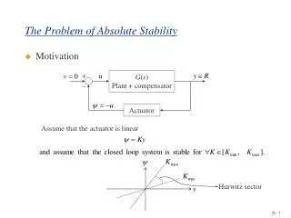
Analysis of Absolute Stability • Figure 4.5 shows a basic regulator system. In this system G(s) is the transfer function of the plant and is equal to C(sI − A)−1B where (A,B, C) is the state variable description of the plant (x is the n-dimensional state vector) • The function Φ(t, y), represents a memory less, possibly time-varying nonlinearity—in our case, the fuzzy controller. • Clearly, the fuzzy controller can be sector-bounded in the same manner as the saturation nonlinearity with either α = 0 for the global case, or for local stability, with some α > 0
Last, we define D(α, β) to be a closed disk in the complex plane whose diameter is the line segment connecting the points −1 α + j0 and −1 β + j0. A picture of thisdisk is shown in Figure 4.7.
Circle Criterion with Sufficient and Necessary Conditions (SNC) For the system of Figure 4.5 with Φ defined as Φ : L2e → L2e, and α,β two given real numbers with α < β, the following two statements are equivalent. 1. The feedback system is L2-stable with finite gain and zero bias for every Φ belonging to the sector (α, β). 2. The transfer function G satisfies one of the following conditions as appropriate: (a) If αβ > 0, then the Nyquist plot of G(jω) does not intersect the interior of the disk D(α, β) and encircles the interior of the disk D(α, β) exactly m times in the counterclockwise direction, where m is the number of poles of G with positive real part. (b) If α = 0, then G has no real poles with positive real part, and Re[G(jω)] ≥ −1 β for all ω. (c) If αβ < 0, then G is a stable transfer function and the Nyquist plot ofG(jω) lies inside the disk D(α, β) for all ω.
1. If 0 < α < β, the Nyquist plot of G(jω) is bounded away from the disk D(α, β) and encircles it m times in the counterclockwise direction where m is the number of poles of G(s) in the open right half-plane. 2. If 0 = α < β, G(s) is Hurwitz (i.e., has its poles in the open left half plane) and the Nyquist plot of G(jω) lies to the right of the line s = −1 β . 3. If α < 0 < β, G(s) is Hurwitz and the Nyquist plot of G(jω) lies in the interior of the disk D(α, β) and is bounded away from the circumference of D(α, β).
Example: Temperature Control • Thermal process shown in Figure 4.8, where τe is the temperature of a liquid entering the insulated chamber, τo is the temperature of the liquid leaving the chamber, and τ = τo − τe is the temperature difference due to the thermal process. The heater/cooling element input is denoted with q. The desired temperature is τd. • Figure 4.9. The controller Gc(s) is a post compensator for the fuzzy controller. Suppose that we begin by choosing Gc(s) = K = 2 and that we simply consider this gain to be part of the plant. Furthermore, for the SISO fuzzy controller we use input membership functions shown in Figure 4.10 and output membership functions shown in Figure 4.11. Note that we denote the variable that is output from the fuzzy controller (and input to Gc(s)) as q.
If e is positive small Then q is positive small • if e is zero Then q is zero • If e is negative big Then q is negative big We use minimum to represent the premise and implication, singleton fuzzification,and COG defuzzification (different from our parameterized fuzzy controller)
Analysis of Steady-State Tracking Error • A terrain-following and terrain-avoidance aircraft control system uses an altimeter to provide a measurement of the distance of the aircraft from the ground to decide how to steer the aircraft to follow the earth at a pilot-specified height. • If a fuzzy controller is employed for such an application, and it consistently seeks to control the height of the plane to be lower than what the pilot specifies, there will be a steady-state tracking error (an error between the desired and actual heights) that could result in a crash
Theory of Tracking Error for Nonlinear Systems • The system is assumed to be of the configuration shown in Figure 4.1 where r, e, u, and y belong to L∞e and Φ(e) is the SISO fuzzy controller • ess = limt→∞ e(t) the steady-state tracking error. G(s) • where ρ, a nonnegative integer, is the number of poles of G(s) at s = 0, and p(s) and sρq(s) are relatively prime polynomials (i.e., they have no common factors) such that deg(p(s)) < deg(sρq(s)
Tracking Error Theorem 1. If r(t) approaches a limit l as t→∞, then ess ≡ limt→∞ e(t) exists. Moreover, ess = 0 if and only if l = 0 and ρ = 0, and then ess = Θ(γ) 2. Assuming that r(t) = ν j=0 ajtj, t ≥0 (4.28) in which the aj are real, ν is a positive integer, and aν = 0, the following holds: (a) e is unbounded if ν > ρ. (b) if ν ≤ ρ, then e approaches a limit as t → ∞. If ν = ρ, this limit is ess = Θ(γ) • An examination of the above theorem reveals that in actuality the proposed method for finding the steady-state error for fuzzy control systems is similar to the equations used in conventional linear control systems
Example: Hydrofoil Controller Design • The HS Denison is an 80-ton hydrofoil stabilized via flaps on the main foils and the incidence of the aft foil. The transfer function for a linearized model of the plant that includes the foil and vehicle is • We first determine that if α = 0, then β must be less than 1.56 for the circlecriterion conditions to be satisfied. Therefore, our preliminary design for the SISO parameterized fuzzy controller will have A = B = 1 • If our input r(t) is a step with magnitude 5.0, then we will use the first condition of the theorem and γ = 3.3333. Using these values in the iterative equation, we find that our steady-state error will be 4.0. • This is a very large error and is obviously 214 Chapter 4 / Nonlinear Analysis much larger than 1%. Even with β = 1.559 we cannot meet the error requirement. Therefore, the system requirements cannot be met with a simple fuzzy controller • Simulations for this system with A = B = 1 show that in fact ess = 0 and we have met the design criteria.