Download
1 / 36
370 likes | 671 Views
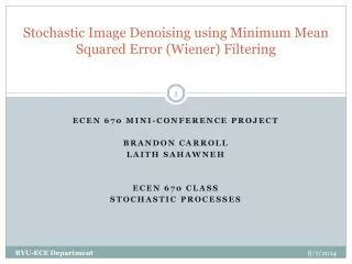
Stochastic Image Denoising using Minimum Mean Squared Error (Wiener) Filtering. ECEN 670 mini-conference Project Brandon Carroll Laith Sahawneh Ecen 670 Class Stochastic Processes. Outline. Introduction Theory: Wiener Filter Derivation Results & Analysis Conclusion. Introduction.

E N D
Stochastic Image Denoising using Minimum MeanSquared Error (Wiener) Filtering ECEN 670 mini-conference Project Brandon Carroll LaithSahawneh Ecen 670 Class Stochastic Processes BYU-ECE Department
Outline • Introduction • Theory: Wiener Filter Derivation • Results & Analysis • Conclusion BYU-ECE Department
Introduction Digital Images (Very brief introduction): • A digital image is generally encoded as a matrix of gray-level or color values. • An image may be defined as a two-dimensional function, x[u,v], where u, v are spatial (plane) coordinates. • In the case of color images, x[u,v] is a triplet of values for the red, green, and blue components BYU-ECE Department
Introduction Example: This is how images represented in computer Color Images BYU-ECE Department
Introduction Image Denoising and Restoration: Image denoising is one of the fundamental challenges in the field of image processing. Employed using variety of configurations in a wide variety of applications: namely: Object recognition, photo enhancement, and image restoration. The objective of image restoration is to improve a given image in some predefined sense. Image restoration attempts to reconstruct or recover a degraded image by using a priori knowledge of the degradation phenomenon. BYU-ECE Department
Introduction • The purpose of image restoration is to restore a degraded/distorted image to its original content and quality. • Image restoration assumes a degradation model that is known or can be estimated. Noise n(u, v) y(u, v) Degradation Function h Restoration Filter (Wiener Filter) x(u, v) x(u, v) ∑ Denoising and Restoration Process Degradation Process with additive noise Linear, space-invariant degradation model: Apply the inverse process to recover the original image ?? BYU-ECE Department
Introduction • Point spread function (PSF) : Convolution Kernel – Impulse Response • What h will give us g = f ? Dirac Delta Function (Unit Impulse) BYU-ECE Department
Optical System point spread function point source Introduction • Point spread function (PSF) : Optical System image scene • An ideal optical system that does not degrade the image at all would have a Dirac delta function as its PSF • However, optical systems are never ideal. • The PSF is the response of the system to a Dirac delta function input. BYU-ECE Department
Introduction • Point spread function (PSF) : • The impulse is a point (or pixel) of light • The impulse response is commonly referred to as the PSF • Impulse of Light • Image (degraded) impulse BYU-ECE Department
Introduction • Noise models • Most types of noise are modeled as probability density functions (PDFs) • Noise model is decided based on understanding of the physics of the sources of noise. • Gaussian: poor illumination • Rayleigh: range image • Gamma, exp: laser imaging • Impulse: faulty switch during imaging, • Uniform: quantization. • Parameters can be estimated based on histogram on small flat area of an image. • De-noising • Spatial filtering (Mean filters, Median, Max, Min …) • Frequency domain filtering ( Inverse Filter, Wiener Filter, …) BYU-ECE Department
Introduction • Estimation of noise parameters: • 1. Gaussian Noise • 2. Uniform Noise • 3. Impulse (Salt& Pepper) Noise BYU-ECE Department
Introduction • Estimation of noise parameters: • The parameters of noise in the spatial domain may be known from the sensors specification or a priori-knowledge of noise distribution. • In most cases it is necessary to estimate these parameters to specify the corresponding noise PDF from sample images being denoised. • How to estimate the noise parameters? The common approach is to select a region of interest (ROI) in an image with as featurelessa background as possible, so that the variability of intensity values in the region will be due primarily to noise! { Let zibe a discrete random variable that denotes intensity levels in an image, and p(zi), i = 1, 2, . . .,L - 1 be the corresponding normalized histogram, where, L is the number of possible intensity values. The histogram component p(zi) is an estimate of the probability of occurrence of intensity value zi.} BYU-ECE Department
Introduction • Estimation of noise parameters: 2. Find the histogram of ROI. 3. Normalized histogram of (ROI) which can be viewed as an approximation of the intensity PDF! 4. Describe the shape of noise PDF via its central moments (estimate the mean and variance and then compute a and b variables if needed). BYU-ECE Department
Introduction • Estimation of noise parameters (Example – Our Matlab Code Simulation): Original Image Normalized histogram of ROI Histogram of ROI Image with Gaussian Noise BYU-ECE Department
Introduction Uniform Noise Histogram Impulse Noise Histogram BYU-ECE Department
Wiener Filter • Image Restoration Approaches • Classical approaches • Algebraic approaches • Unconstrained optimization • Inverse filter • Constrained optimization • Weiner filter • The regularization theory BYU-ECE Department
Wiener Filter • Inverse Filter: Noise n(u, v) y(u, v) Degradation Function h Restoration Filter (Wiener Filter) x(u, v) x(u, v) ∑ Denoising and Restoration Process Degradation Process with additive noise BYU-ECE Department
Wiener Filter • Wiener Filter: • Most neighboring pixels are highly correlated, while widely separated pixels are only loosely correlated. • Therefore, the autocorrelation function of typical images generally decreases away from the origin. • Power spectrum = Fourier transform of autocorrelation, therefore the power spectrum of an image generally decreases with frequency. • Typical noise sources have either a flat power spectrum or one that decreases with frequency more slowly than typical image power spectrum. • Therefore, the signal should dominate at low frequencies, while the noise dominates athigh frequencies. BYU-ECE Department
Wiener Filter • Wiener Filter: • Assumptions: The noise and the image are uncorrelated. Either the noise or the image is zero-mean, and that the intensities in the estimate are a linear function of the intensities in the noisy image. It also assumes that the power spectrum of both the noise and the original image are known • Theory (Derivation) • Degradation model BYU-ECE Department
Wiener Filter • The Goal • We wish to find an LTI filter with impulse response g[u, v] that gives us the MMSE estimate of x[u, v]: • The MSE is given by: Parseval’s theorem states: Since they are directly proportional, we can minimize the spatial domain mean squared error by minimizing the frequency domain mean squared error: Using property of the Fourier transform: Substitute in Y then rearrange the terms BYU-ECE Department
Wiener Filter Using the definition of an absolute square, we get: Multiplying out the terms and distributing the expected value across the sums We assume that the noise is independent of the original image and that either the noise or the image is zero-mean: Where the power spectral densities are defined as: BYU-ECE Department
Wiener Filter To find the G that minimizes the MSE, we take the derivative with respect to G(fu,fv): HH* = │H│2 Solving for G* gives: Finally, we write the equation in terms of the signal-to-noise Ratio: BYU-ECE Department
Wiener Filter Wiener Filter Equation: Arranged intuitively: BYU-ECE Department
Results & Analysis Original image 20 pixel motion blur BYU-ECE Department
Results & Analysis Original image 20 pixel motion blur, inverse filtered BYU-ECE Department
Results & Analysis Original image 5 pixel motion blur, imperceptible Gaussian noise BYU-ECE Department
Results & Analysis Original image 5 pixel motion blur, imperceptible Gaussian noise, inverse filtered BYU-ECE Department
Results & Analysis Original image 5 pixel motion blur, imperceptible Gaussian noise, Wiener filtered BYU-ECE Department
Results & Analysis Original image 15 pixel motion blur, Gaussian noise BYU-ECE Department
Results & Analysis 15 pixel motion blur, Gaussian noise 15 pixel motion blur, Gaussian noise, inverse filtered BYU-ECE Department
Results & Analysis 15 pixel motion blur, Gaussian noise 15 pixel motion blur, Gaussian noise, Wiener filtered BYU-ECE Department
Results & Analysis 3 pixel motion blur, salt and pepper noise 3 pixel motion blur, salt and pepper noise, inverse filtered BYU-ECE Department
Results & Analysis 3 pixel motion blur, salt and pepper noise 3 pixel motion blur, salt and pepper noise, Wiener filtered BYU-ECE Department
Results & Analysis Wiener filter using actual noise spectrum Wiener filter using estimated noise spectrum Region of Interest BYU-ECE Department
Conclusions • Inverse filter works well with no noise • Wiener filter performs much better in the presence of noise • Assumes knowledge of degradation function (a common requirement for image restoration algorithms) • Assumes knowledge of the power spectra of the noise and original image (less common, makes it less useful) • The noise power spectrum can be effectively estimated by analyzing the histogram of an ROI in the noisy image • Forms the basis of other more robust restoration approaches BYU-ECE Department
Thank you BYU-ECE Department