Topological Sorting and Least-cost Path Algorithms
170 likes | 439 Views
Topological Sorting and Least-cost Path Algorithms. undershorts. socks. watch. pants. shoes. shirt. belt. tie. jacket. Topological Sort. Topological sort of a dag G = (V, E) Linear ordering A of all vertices from V If edge ( u,v ) E => A[u] < A[v].

Topological Sorting and Least-cost Path Algorithms
E N D
Presentation Transcript
undershorts socks watch pants shoes shirt belt tie jacket Topological Sort • Topological sort of a dag G = (V, E) • Linear ordering A of all vertices from V • If edge (u,v) E => A[u] < A[v] socks, undershorts, pants, shoes, watch, shirt, belt, tie, jacket
|V| |V| But this is O( |V|2 )
Topological Sort • Uses DFS • Topological-Sort (G) • Call DFS (G) to compute finishing times f[v] for each v • Output vertices in decreasing order of finishing time • Time complexity • O (|V| + |E|)
17, 18 11, 16 12, 15 13, 14 9, 10 1, 8 undershorts socks 6, 7 watch 2, 5 pants shoes 3, 4 shirt belt tie jacket Example 18-socks, 16-undershorts, 15-pants, 14-shoes, 10-watch, 8-shirt, 7-belt, 5-tie, 4-jacket
Correctness • Theorem • Topological-Sort(G) produces a topological sort of a directed acyclic graph G • Proof: • Consider any edge (u, v) • Suffices to show f[v] < f[u] • Three possible types of edges • Tree edge, forward edge, cross edge
Single-Source Shortest Path • Problem: given a weighted directed graph G, find the minimum-cost path from a given source vertex s to every other vertex v • “Shortest-path” = minimum weight • Weight of path is sum of edges • E.g., a road map: what is the shortest path from Millersville to Wrightsville?
Dijkstra’s Algorithm • Cannot have negative edge weights • Similar to breadth-first search • Grow a tree gradually, advancing from vertices taken from a queue (priority queue instead of normal queue) • Also similar to Prim’s algorithm for MST • Use a priority queue keyed on d[v]
B 2 10 A 4 3 D 5 1 C What will be the total running time?
B 2 10 A 4 3 D 5 1 C RelaxationStep Note: thisis really a call to Q->DecreaseKey() for a priority queue Q Dijkstra’s Algorithm Dijkstra(G) for each v V d[v] = ; d[s] = 0; S = ; Q = V; while (Q ) u = ExtractMin(Q); S = S U {u}; for each v u->Adj[] if (d[v] > d[u]+w(u,v)) d[v] = d[u]+w(u,v); p[v] = u;
Dijkstra’s Algorithm Dijkstra(G) for each v V d[v] = ; d[s] = 0; S = ; Q = V; while (Q ) u = ExtractMin(Q); S = S U {u}; for each v u->Adj[] if (d[v] > d[u]+w(u,v)) d[v] = d[u]+w(u,v); p[v] = u; How many times is ExtractMin() called? O(V lg V) How many times is DecreaseKey() called? O(E lg V) What will be the total running time? O(E lgV + V lg V) = O(E lg V) since E <= V2
2 2 9 6 5 5 Relax Relax 2 2 7 6 5 5 Relaxation • Key operation: relaxation • Let (u,v) be cost of shortest path from u to v • Maintain upper bound d[v] on (s,v): Relax(u,v,w) { if (d[v] > d[u]+w) then { d[v]=d[u]+w; p[v] = u; } } } w w v v u u u v u v
Initialize d[], which will converge to shortest-path value Relaxation: Make |V|-1 passes, relaxing each edge Test for solution: have we converged yet? Ie, negative cycle? Bellman-Ford Algorithm BellmanFord() for each v V d[v] = ; d[s] = 0; for i=1 to |V|-1 { for each edge (u,v) E Relax(u,v, w(u,v)); } for each edge (u,v) E if (d[v] > d[u] + w(u,v)) return “no solution”; Relax(u,v,w): if (d[v] > d[u]+w) then d[v]=d[u]+w
Bellman-Ford Algorithm BellmanFord() for each v V d[v] = ; d[s] = 0; for i=1 to |V|-1 for each edge (u,v) E Relax(u,v, w(u,v)); for each edge (u,v) E if (d[v] > d[u] + w(u,v)) return “no solution”; Relax(u,v,w): if (d[v] > d[u]+w) then d[v]=d[u]+w What will be the running time?
Bellman-Ford • Running time: O(VE) • Not so good for large dense graphs • But a very practical algorithm in many ways • Note that order in which edges are processed affects how quickly it converges • A distributed variant of the Bellman–Ford algorithm is used in distance-vector routing protocols