Sorting Algorithms

1. Sorting Algorithms Ananth Grama, Anshul Gupta, George Karypis, and Vipin Kumar To accompany the text ``Introduction to Parallel Computing'', Addison Wesley, 2003.

2. Topic Overview • Issues in Sorting on Parallel Computers • Sorting Networks • Bubble Sort and its Variants • Quicksort • Bucket and Sample Sort • Other Sorting Algorithms

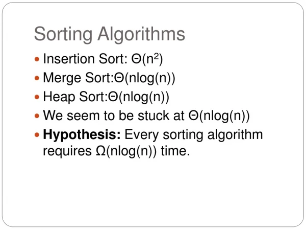
3. Sorting: Overview • One of the most commonly used and well-studied kernels. • Sorting can be comparison-based or noncomparison-based. • The fundamental operation of comparison-based sorting is compare-exchange. • The lower bound on any comparison-based sort of n numbers is Θ(nlog n) . • We focus here on comparison-based sorting algorithms.

4. Sorting: Basics What is a parallel sorted sequence? Where are the input and output lists stored? • We assume that the input and output lists are distributed. • The sorted list is partitioned with the property that each partitioned list is sorted and each element in processor Pi's list is less than that in Pj's list if i < j.

5. Sorting: Parallel Compare Exchange Operation A parallel compare-exchange operation. Processes Pi and Pj send their elements to each other. Process Pi keeps min{ai,aj}, and Pj keeps max{ai, aj}.

6. Sorting: Basics What is the parallel counterpart to a sequential comparator? • If each processor has one element, the compare exchange operation stores the smaller element at the processor with smaller id. This can be done in ts + tw time. • If we have more than one element per processor, we call this operation a compare split. Assume each of two processors have n/p elements. • After the compare-split operation, the smaller n/p elements are at processor Pi and the larger n/p elements at Pj, where i < j. • The time for a compare-split operation is (ts+ twn/p), assuming that the two partial lists were initially sorted.

7. Sorting: Parallel Compare Split Operation A compare-split operation. Each process sends its block of size n/p to the other process. Each process merges the received block with its own block and retains only the appropriate half of the merged block. In this example, process Pi retains the smaller elements and process Pi retains the larger elements.

8. Sorting Networks • Networks of comparators designed specifically for sorting. • A comparator is a device with two inputs x and y and two outputs x' and y'. For an increasing comparator, x' = min{x,y} and y' = min{x,y}; and vice-versa. • We denote an increasing comparator byand a decreasing comparator by Ө. • The speed of the network is proportional to its depth.

9. Sorting Networks: Comparators A schematic representation of comparators: (a) an increasing comparator, and (b) a decreasing comparator.

10. Sorting Networks A typical sorting network. Every sorting network is made up of a series of columns, and each column contains a number of comparators connected in parallel.

11. Sorting Networks: Bitonic Sort • A bitonic sorting network sorts n elements in Θ(log2n) time. • A bitonic sequence has two tones - increasing and decreasing, or vice versa. Any cyclic rotation of such networks is also considered bitonic. • 1,2,4,7,6,0 is a bitonic sequence, because it first increases and then decreases. 8,9,2,1,0,4 is another bitonic sequence, because it is a cyclic shift of 0,4,8,9,2,1. • The kernel of the network is the rearrangement of a bitonic sequence into a sorted sequence.

12. Sorting Networks: Bitonic Sort • Let s = a0,a1,…,an-1 be a bitonic sequence such that a0 ≤ a1 ≤ ··· ≤ an/2-1 and an/2 ≥an/2+1 ≥ ··· ≥ an-1. • Consider the following subsequences of s: s1 = min{a0,an/2},min{a1,an/2+1},…,min{an/2-1,an-1} s2 = max{a0,an/2},max{a1,an/2+1},…,max{an/2-1,an-1} (1) • Note that s1 and s2 are both bitonic and each element of s1 is less than every element in s2. • We can apply the procedure recursively on s1 and s2 to get the sorted sequence.

13. Sorting Networks: Bitonic Sort Merging a 16-element bitonic sequence through a series of log 16 bitonic splits.

14. Sorting Networks: Bitonic Sort • We can easily build a sorting network to implement this bitonic merge algorithm. • Such a network is called a bitonic merging network. • The network contains log n columns. Each column contains n/2 comparators and performs one step of the bitonic merge. • We denote a bitonic merging network with n inputs by BM[n]. • Replacing the  comparators by Ө comparators results in a decreasing output sequence; such a network is denoted by ӨBM[n].

15. Sorting Networks: Bitonic Sort A bitonic merging network for n = 16. The input wires are numbered 0,1,…, n - 1, and the binary representation of these numbers is shown. Each column of comparators is drawn separately; the entire figure represents a BM[16] bitonic merging network. The network takes a bitonic sequence and outputs it in sorted order.

16. Sorting Networks: Bitonic Sort How do we sort an unsorted sequence using a bitonic merge? • We must first build a single bitonic sequence from the given sequence. • A sequence of length 2 is a bitonic sequence. • A bitonic sequence of length 4 can be built by sorting the first two elements using BM[2] and next two, using ӨBM[2]. • This process can be repeated to generate larger bitonic sequences.

17. Sorting Networks: Bitonic Sort A schematic representation of a network that converts an input sequence into a bitonic sequence. In this example, BM[k] and ӨBM[k] denote bitonic merging networks of input size k that use  and Ө comparators, respectively. The last merging network (BM[16]) sorts the input. In this example, n = 16.

18. Sorting Networks: Bitonic Sort The comparator network that transforms an input sequence of 16 unordered numbers into a bitonic sequence.

19. Sorting Networks: Bitonic Sort • The depth of the network is Θ(log2n). • Each stage of the network contains n/2 comparators. A serial implementation of the network would have complexity Θ(nlog2n).

20. Mapping Bitonic Sort to Hypercubes • Consider the case of one item per processor. The question becomes one of how the wires in the bitonic network should be mapped to the hypercube interconnect. • Note from our earlier examples that the compare-exchange operation is performed between two wires only if their labels differ in exactly one bit! • This implies a direct mapping of wires to processors. All communication is nearest neighbor!

21. Mapping Bitonic Sort to Hypercubes Communication during the last stage of bitonic sort. Each wire is mapped to a hypercube process; each connection represents a compare-exchange between processes.

22. Mapping Bitonic Sort to Hypercubes Communication characteristics of bitonic sort on a hypercube. During each stage of the algorithm, processes communicate along the dimensions shown.

23. Mapping Bitonic Sort to Hypercubes Parallel formulation of bitonic sort on a hypercube with n = 2d processes.

24. Mapping Bitonic Sort to Hypercubes • During each step of the algorithm, every process performs a compare-exchange operation (single nearest neighbor communication of one word). • Since each step takes Θ(1) time, the parallel time is Tp = Θ(log2n) (2) • This algorithm is cost optimal w.r.t. its serial counterpart, but not w.r.t. the best sorting algorithm.

25. Mapping Bitonic Sort to Meshes • The connectivity of a mesh is lower than that of a hypercube, so we must expect some overhead in this mapping. • Consider the row-major shuffled mapping of wires to processors.

26. Mapping Bitonic Sort to Meshes Different ways of mapping the input wires of the bitonic sorting network to a mesh of processes: (a) row-major mapping, (b) row-major snakelike mapping, and (c) row-major shuffled mapping.

27. Mapping Bitonic Sort to Meshes The last stage of the bitonic sort algorithm for n = 16 on a mesh, using the row-major shuffled mapping. During each step, process pairs compare-exchange their elements. Arrows indicate the pairs of processes that perform compare-exchange operations.

28. Mapping Bitonic Sort to Meshes • In the row-major shuffled mapping, wires that differ at the ith least-significant bit are mapped onto mesh processes that are 2(i-1)/2 communication links away. • The total amount of communication performed by each process is . The total computation performed by each process is Θ(log2n). • The parallel runtime is: • This is not cost optimal.

29. Block of Elements Per Processor • Each process is assigned a block of n/p elements. • The first step is a local sort of the local block. • Each subsequent compare-exchange operation is replaced by a compare-split operation. • We can effectively view the bitonic network as having (1 + log p)(log p)/2 steps.

30. Block of Elements Per Processor: Hypercube • Initially the processes sort their n/p elements (using merge sort) in time Θ((n/p)log(n/p)) and then perform Θ(log2p) compare-split steps. • The parallel run time of this formulation is • Comparing to an optimal sort, the algorithm can efficiently use up toprocesses. • The isoefficiency function due to both communication and extra work is Θ(plog plog2p) .

31. Block of Elements Per Processor: Mesh • The parallel runtime in this case is given by: • This formulation can efficiently use up to p = Θ(log2n) processes. • The isoefficiency function is

32. Performance of Parallel Bitonic Sort The performance of parallel formulations of bitonic sort for n elements on p processes.

33. Bubble Sort and its Variants The sequential bubble sort algorithm compares and exchanges adjacent elements in the sequence to be sorted: Sequential bubble sort algorithm.

34. Bubble Sort and its Variants • The complexity of bubble sort is Θ(n2). • Bubble sort is difficult to parallelize since the algorithm has no concurrency. • A simple variant, though, uncovers the concurrency.

35. Odd-Even Transposition Sequential odd-even transposition sort algorithm.

36. Odd-Even Transposition Sorting n = 8 elements, using the odd-even transposition sort algorithm. During each phase, n = 8 elements are compared.

37. Odd-Even Transposition • After n phases of odd-even exchanges, the sequence is sorted. • Each phase of the algorithm (either odd or even) requires Θ(n) comparisons. • Serial complexity is Θ(n2).

38. Parallel Odd-Even Transposition • Consider the one item per processor case. • There are n iterations, in each iteration, each processor does one compare-exchange. • The parallel run time of this formulation is Θ(n). • This is cost optimal with respect to the base serial algorithm but not the optimal one.

39. Parallel Odd-Even Transposition Parallel formulation of odd-even transposition.

40. Parallel Odd-Even Transposition • Consider a block of n/p elements per processor. • The first step is a local sort. • In each subsequent step, the compare exchange operation is replaced by the compare split operation. • The parallel run time of the formulation is

41. Parallel Odd-Even Transposition

42. Parallel Odd-Even Transposition • The parallel formulation is cost-optimal if p = O(log n). • The isoefficiency function of this parallel formulation is Θ(p2p). • The isoefficiency function determines the ease with which a parallel system can maintain a constant efficiency and hence achieve speedups increasing in proportion to the number of processing elements. A small isoefficiency function means that small increments in the problem size are sufficient for the efficient utilization of an increasing number of processing elements, indicating that the parallel system is highly scalable. However, a large isoefficiency function indicates a poorly scalable parallel system. The isoefficiency function does not exist for unscalable parallel systems, because in such systems the efficiency cannot be kept at any constant value as p increases, no matter how fast the problem size is increased.

43. Shellsort • Let n be the number of elements to be sorted and p be the number of processes. • During the first phase, processes that are far away from each other in the array compare-split their elements. • During the second phase, the algorithm switches to an odd-even transposition sort.

44. Parallel Shellsort • Initially, each process sorts its block of n/p elements internally. • Each process is now paired with its corresponding process in the reverse order of the array. That is, process Pi, where i < p/2, is paired with process Pp-i-1. • A compare-split operation is performed. • The processes are split into two groups of size p/2 each and the process repeated in each group.

45. Parallel Shellsort An example of the first phase of parallel shellsort on an eight-process array.

46. Parallel Shellsort • Each process performs d = log p compare-split operations. • With O(p) bisection width, each communication can be performed in time Θ(n/p) for a total time of Θ((nlog p)/p). • In the second phase, l odd and even phases are performed, each requiring time Θ(n/p). • The parallel run time of the algorithm is:

47. Quicksort • Quicksort is one of the most common sorting algorithms for sequential computers because of its simplicity, low overhead, and optimal average complexity. • Quicksort selects one of the entries in the sequence to be the pivot and divides the sequence into two - one with all elements less than the pivot and other greater. • The process is recursively applied to each of the sublists.

48. Quicksort The sequential quicksort algorithm.

49. Quicksort Example of the quicksort algorithm sorting a sequence of size n = 8.

50. Quicksort • The performance of quicksort depends critically on the quality of the pivot. • In the best case, the pivot divides the list in such a way that the larger of the two lists does not have more than αnelements (for some constant α). • In this case, the complexity of quicksort is O(nlog n).