Download
1 / 44
440 likes | 555 Views
Reconstruction of Solar EUV Flux in Centuries Past. Leif Svalgaard Stanford University Big Bear Solar Observatory 23 rd Sept. 2014 NSO, Sunspot, NM 3 rd Oct. 2014. The Effect of Solar EUV.

E N D
Reconstruction of Solar EUV Flux in Centuries Past Leif Svalgaard Stanford University Big Bear Solar Observatory 23rd Sept. 2014 NSO, Sunspot, NM 3rd Oct. 2014
The Effect of Solar EUV The EUV causes an observable variation of the geomagnetic field at the surface through a complex chain of physical connections. The physics of each link in the chain is well-understood in quantitative detail and can be successfully modeled. We’ll use this chain in reverse to deduce the EUV flux from the geomagnetic variation.
Ionospheric Layers An effective dynamo process takes place in the dayside E-layer where the density, both of the neutral atmosphere and of the electrons are high enough. The geomagnetic response is thus due to electric currents induced in the E-layer.
Electron Density due to EUV The conductivity at a given height is proportional to the electron number density Ne. In the dynamo region the ionospheric plasma is largely in photochemical equilibrium. The dominant plasma species is O+2, which is produced by photo ionization at a rate J (s−1) and lost through recombination with electrons at a rate α (s−1), producing the Airglow. < 102.7 nm The rate of change of the number of ions Ni, dNi/dt and in the number of electrons Ne, dNe/dt are given by dNi/dt = J cos(χ) - αNiNe and dNe/dt = J cos(χ) - αNeNi. Because the process is slow (the Zenith angle χchanges slowly) we have a quasi steady-state, in which there is no net electric charge, so Ni = Ne = N. In a steady-state dN/dt = 0, so the equations can be written 0 = J cos(χ) - αN2, and so finally N =√(Jα-1cos(χ)), (the Chapman Function, first derived by Sidney Chapman). Since the conductivity, Σ, depends on the number of electrons N, we expect that Σ scales with the square root √(J) of the overhead EUV flux with λ < 102.7 nm.
Magnitude of Magnetic Effect The magnitude, A, of the variation of the East Component due to the dynamo process is given by A = ¾ μoΣ U Bz where μo is the permeability of the vacuum (4π× 107), Σ is the effective ionospheric conductivity (S), U is zonal neutral wind speed (m s−1), and Bz is the vertical geomagnetic field strength (nT). In the E-layer the conductivity is a tensor and highly anisotropic. To first approximation Σ depends on N and inversely on B: Σ ~ N/B, such that the magnitude A only depends on the electron density and the zonal neutral wind speed. The cancellation of B is not perfect, though, depending on the precise geometry of the field. In addition, the ratio between internal and external current intensity varies with location. The net result is that A can vary somewhat from location to location even for given N and U. Thus a normalization of the response to a reference location is necessary
The E-layer Current System North X . rY Morning H rD Evening D East Y Y = H sin(D) dY = H cos(D) dD For small dD A current system in the ionosphere is created and maintained by solar EUV radiation The magnetic effect of this system was discovered by George Graham in 1722
The Magnetic Signal at Midlatitudes X Y Z Geomagnetic Observatories The effect in the Y-component is rather uniform for latitudes between 20º and 60º
The Diurnal Variation of the Declination for Low, Medium, and High Solar Activity rY = H cos D rD
PSM-POT-VLJ-SED-CLF-NGK A ‘Master’ record can now be build by averaging the German and French chains. We shall normalize all other stations to this Master record.
Adding Prague back to 1840 If the regression against the Master record is not quite linear, a power law is used.
Variometer Invented by Gauss, 1833 Helsinki 1844-1912 Nevanlinna et al.
Classic Method since 1847 Magnetic Recorders Classic Instruments circa 1900 Modern Instrument
And So On: For 107 Geomagnetic Observatories with Good Data Next slide shows all [normalized] stations in a combined graph
N Std Dev.
Composite rY Series 1840-2014 From the Standard Deviation and the Number of Station in each Year we can compute the Standard Error of the Mean and plot the ±1-sigma envelope
The Effect of Solar EUV The EUV causes an observable variation of the geomagnetic field at the surface through a complex chain of physical connections. The physics of each link in the chain is well-understood in quantitative detail and can be successfully modeled. We’ll use this chain in reverse to deduce the EUV flux from the geomagnetic variation.
EUV Bands and Solar Spectrum Most of the Energetic Photons are in the 0.1-50 nm Band /nm SOHO-SEM 0.1-50 nm 102.7 nm for O2
We Correct the SEM-series for Degradation Comparing with F10.7 and Mg II Indices Mg II F10.7
rY and F10.71/2 and EUV1/2 Since 1996 Since 1996 Since 1947
Reconstructed EUV Flux 1840-2014 This is, I believe, an accurate depiction of true solar activity since 1840
We can compare that with the Zurich Sunspot Number Wolfer & Brunner 1 spot Locarno 2014-9-22 2 spots
Recent Drift of International Sunspot Number k-values Plot of different multi-station average k ratios spanning the 1955–2013 interval, for 4 different subsets of stations (A: 3 best stations; B: 6 stations; C: 16 stations; D: 22 stations). Effect is under way to re-examine the International Sunspot Number: Clette et al., Space Science Reviews, 2014
How About the Group Sunspot Number? The main issue with the GSN is a change relative to the ZSN during 1880-1900. This is mainly caused by a drift in the reference count of the standard (Royal Greenwich Observatory) The ratio between the Group Sunspot Number reveals two major problem areas. We can now identify the cause of each ZSN issue GSN issue
RGO Groups/Sunspot Groups Early on RGO counts fewer groups than Sunspot Observers
Rudolf Wolf Discovered the Effect in 1852. Today We Know the Cause A.C. Young: The Sun (revised edition, 1897).
Observations in the 1740s Olof Petrus Hjorter was married to Anders Celsius’ sister and made more than 10,000 observations of the magnetic declination in the 1740s. The data is available and I’m trying to find time to work on them. Hjorter’s measurements of the magnetic declination at Uppsala during April 8-12 1741 (old style). The curve shows the average variation of the magnetic declination during April 1997 at nearby Lovö (Sweden).
Observations in the 1760s John Canton [1759] made ~4000 observations of the Declination on 603 days and noted that 574 of these days showed a ‘regular’ variation, while the remainder (on which aurorae were ‘always’ seen) had an ‘irregular’ diurnal variation.
Observations in 1787-1805 George Gilpin sailed on the Resolution during Cook's second voyage as assistant to William Wales, the astronomer. Gilpin was elected Clerk and Housekeeper for the Royal Society of London on 03 March 1785 and remained in these positions until his death in 1810.
Wolf’s Series of Declination Ranges Next Task: to critically resolve the discrepancy (in oval)
The Effect of Solar EUV The EUV causes an observable variation of the geomagnetic field at the surface through a complex chain of physical connections. The physics of each link in the chain is well-understood in quantitative detail and can be successfully modeled. We’ll use this chain in reverse to deduce the EUV flux from the geomagnetic variation.
Progress in Reconstructing Solar Wind Magnetic Field back to 1840s Svalgaard 2014 Using u-measure Even using only ONE station, the ‘IDV’ signature is strong enough to show the effect
Schwadron et al. (2010) HMF B Modelwith my set of parameters with a ‘Floor’ von Neumann: “with four parameters I can fit an elephant, and with five I can make him wiggle his trunk” This model has about eight parameters… B = 4+ 0.318 SSNc1/2
HMF B Scales with the Sqrt of the EUV flux B2 ~ EUV Flux
‘Burning Prairie’ => Magnetism Foukal & Eddy, Solar Phys. 2007, 245, 247-249
Conclusions • We can reconstruct with confidence the solar EUV flux [and its proxy F10.7] back to 1840 • The reconstructed EUV flux confirms the discontinuities in the Sunspot Records reported by Clette et al., 2014 • There is more geomagnetic data earlier than 1840, and it now seems important to acquire and process the earlier data. • The EUV flux is concordant with the revised Sunspot Number and the Solar Wind Magnetic Flux • There is no Modern Grand Solar Maximum • Some of this may still be controversial. Aggressive and serious opposition is welcome
Abstract Solar EUV creates the conducting E-layer of the ionosphere, mainly by photo ionization of molecular Oxygen, governed by the so-called Chapman function. Solar heating of the ionosphere creates thermal winds which by dynamo action induce an electric field driving an electric current having a magnetic effect observable on the ground, as was discovered by G. Graham in 1722. The current rises and sets with the Sun and thus causes a readily observable diurnal variation of the geomagnetic field, allowing us the deduce the conductivity and thus the EUV flux as far back as reliable magnetic data reach. High quality data go back to the 1840s and less reliable, but still usable, data are available for the hundred years before that. R. Wolf and, independently, J-A. Gautier discovered the dependence of the diurnal variation on solar activity, and today we understand and can invert that relationship to construct a reliable record of the EUV flux from the geomagnetic record. We compare that to the F10.7 flux and the sunspot number, and find that the reconstructed EUV flux reproduces the F10.7 flux with great accuracy and that the EUV flux clearly shows the discontinuities of the sunspot record identified by Clette et al, 2014.