High-Resolution Sea Ice Motions from AMSR-E Imagery

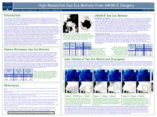
1. 44A078 High-Resolution Sea Ice Motions from AMSR-E Imagery http://nsidc.org Walter N. Meier and Mingrui Dai (Correspondence: walt@nsidc.org) Introduction AMSR-E Sea Ice Motions U Sea ice motion is a key component in the evolution of the sea ice cover. Changes in large-scale sea ice circulation induced by the Arctic Oscillation have been theorized to be an important factor in the recent extreme summer minimums of the 1990s and 2001-2005 (Stroeve et al., 2005) by advecting thicker multiyear ice out of the Arctic and pre-conditioning the basin with thinner ice more susceptible to melt during the following summer (Rigor et al., 2002). Dynamics also affect the sea ice on small scales through the creation of open water (leads and polynyas) and ridging. Sea ice motion has been one of the most common parameters used for assimilation into sea ice models. The assimilated ice motions have been shown to improve model estimates of motion and other related parameters, such as ice thickness (Meier et al., 2000; Zhang et al., 2003). Observations from in situ buoys or Radarsat imagery provide detailed high-resolution ice motion information. However, their utility for data assimilation is limited due their sparse spatial or temporal coverage. Imagery from passive microwave sensors has provided a long history (since 1978) of daily, basin-scale motion estimates in nearly all-sky conditions, but at a coarse spatial resolution. The new Advanced Microwave Scanning Radiometer for EOS (AMSR-E) sensor on the NASA Aqua platform is able to obtain more accurate and more detailed motion estimates than its predecessor, the Special Sensor Microwave/Imager (SSM/I). With more detailed and frequent motion information, important smaller-scale processes, such as lead formation and ridging, can be better characterized. Sea ice models are becoming more sophisticated (e.g., improved rheologies, higher resolution) and new modeling approaches (e.g., Lagrangian particle models) are being developed. The improved sea ice observations from AMSR-E will be particularly beneficial for such models. Here, we evaluate AMSR-E motions from 2003-2004 and demonstrate their potential to yield detailed ice motion estimates as well as estimates of divergence and other parameters relevant to sea ice processes. Evaluation of Motions: AMSR-E is suitable for producing maps of the basin-scale circulation (Figure 1). Several studies have evaluated passive microwave ice motions using alternative sources, particularly buoys (e.g., Agnew et al., 1997; Kwok et al., 1998; Meier et al., 2000). Here, we evaluate the AMSR-E motions during the winter, October 2003 – April 2004 using buoy observations obtained from the International Arctic Buoy Program (IABP) (Rigor and Ortmeyer, 2003). Motion statistics for the Arctic motion fields, derived from coincident observations during October 2003 – April 2004 shows the errors of the passive microwave motions relative to buoy motions (Table 2). The buoy motions have an estimated RMS error of ~0.05 km day-1, and are thus a reasonable “truth” for evaluation of the other motions. Surprisingly, the AMSR-E 36.5 GHz frequency yields motions with comparable errors to the 89 GHz channel. This is likely due to (1) less atmospheric contribution at 36.5 GHz, and (2) limited improvement of oversampling for 89 GHz compared to 36.5 GHz. There is little difference between the horizontally and vertically polarized channels Interpolated Motions:More complete and more accurate ice motion fields can be achieved by combining all sources of passive microwave derived ice motions. Here an optimal interpolation (OI) method is employed to create interpolated fields during March 2004. OI combines the observations based on the error characteristics and the spatial distribution of the estimates to create statistically optimal (minimum error) interpolated fields. This method has also been used in an assimilation mode to combine observed ice motions with estimates from sea ice models (e.g., Meier et al., 2000; Zhang et al., 2003). By combining passive microwave sources, the interpolated fields have a lower bias and RMS error over all each of the individual PM fields (Table 3). V Figure 1. Left: Arctic mean motion for March 2004; Right: Antarctic mean motion for August 2004. The U and V orientation is denoted in the Arctic image, along with the case study area (yellow box). Note the difference in the scale vectors in the bottom right of each image. Table 3. Mean motion error statistics for passive microwave and interpolated motion fields, relative to buoy estimates during March 2004. Passive microwave motions from horizontally polarized imagery. Passive Microwave Sea Ice Motions Table 2. Mean motion error statistics for U and V components from AMSR-E channels, relative to buoy estimates (see Figure 1 for orientation of motion fields). Sea ice motion can be detected with passive microwave imagery using cross-correlation techniques where features in a gridded image are matched in a subsequent, spatially coincident, image (Emery et al., 1991). The motion is computed from the number of pixels separating the feature, the pixel resolution, and the time between images. Oversampling methods can yield subpixel motions. SSM/I 85 GHz brightness temperatures (Tb) have been most commonly used because historically they have had the highest gridded spatial resolution (Table 1). However, at the 85 GHz frequency atmospheric emission can result in uncertainties. Atmospheric emission is typically much lower at the SSM/I 37 GHz frequency, but the spatial resolution is only about half of the 85 GHz channels, thus limiting the motion that it can resolve. The AMSR-E represents a substantial advancement in passive microwave remote sensing technology. Most relevant here is a doubling of the gridded resolution compared to SSM/I. In fact, the effective resolution (the satellite footprint) is even more than double SSM/I (Table 1). Information and AMSR-E and SSM/I Tb data is available from the National Snow and Ice Data Center (http://nsidc.org). Case Studies of Sea Ice Motion and Divergence The three case studies below illustrate the capabilities of the interpolated AMSR-E and SSM/I motions. The region of the case studies is indicated by the boxed region in Figure 1 above. Each case includes the pair of consecutive daily 89 GHz brightness temperature (Tb) images (A, B) used to derive the ice motion field (C). Though computed at every 6.25 grid point, motion vectors are plotted every 150 km for clarity. Warmer Tbs, indicating open water or thin ice are lighter. The ice motion field is repeated with the divergence overlaid (at 6.25 km resolution) over the region of interest (D). The primary feature of interest for each case is circled in yellow. Other deformation fields such as shear and vorticity, though not shown here, can also be calculated. 29 Feb 1 Mar 2 Mar 3 Mar 8 Mar 9 Mar 2004 240 K A B A A B B Table 1. Resolution of SSM/I and AMSR-E Tbs at frequencies used to derive ice motions. Note that the gridded resolution of SSM/I is underspampled (gridded resolution smaller than the footprint) while the gridded AMSR-E is not substantially undersampled. AMSR-E 89 GHz Tb 160 K D C C D Div C D Alaska 20 cm s-1 References Motion/Divergence Agnew, T., H. Le, and T. Hirose, 1997. Estimation of large scale sea ice motion from SSM/I 85.5 GHz imagery, Ann. Glaciol., 25, 305-311. Emery, W.J., C.W. Fowler, J. Hawkins, and R.H. Preller, 1991. Fram Strait satellite image-derived ice motions, J. Geophys. Res., 96(C5), 8917-8920. Kwok, R., A. Schweiger, D.A. Rothrock, S. Pang, and C. Kottmeier, 1998. Sea ice motion from satellite passive microwave imagery assessed with ERS SAR and buoy motions, J. Geophys. Res., 103, 8191-8214. Meier, W.N., J.A. Maslanik, and C. Fowler, 2000. Error analysis and assimilation of remotely sensed ice motion within an Arctic sea ice model, J. Geophys. Res., 105(C2), 3339-3356. Serreze, M.C., J. Maslanik, T.A. Scambos, F. Fetterer, J. Stroeve, K. Knowles, C. Fowler, S. Drobot, R.G. Barry, and T.M. Haran, 2003. A record minimum Arctic sea ice extent and area in 2002, Geophys. Res. Lett., 30(3), 1110, doi: 10.1029/2002GL016406. Stroeve, J.C., M.C. Serreze, F. Fetterer, T. Arbetter, W. Meier, J. Maslanik, and K. Knowles, 2005. Tracking the Arctic’s shrinking ice cover: Another extreme minimum in 2004, Geophys. Res. Lett., 32, L04501, doi: 10.1029/2004GL021810. Rigor, I.G., and M. Ortmeyer, The International Arctic Buoy Programme (IABP), Proc. Eos Trans. AGU, 84 (46), Fall Meet. Suppl., Abstract C41C-0987, Dec. 2003. Rigor, I.G., J.M. Wallace, and R.L. Colony, 2002. Response of sea ice to the Arctic Oscillation, J. Climate, 15, 2648-2663. Zhang, J., D.R. Thomas, D.A. Rothrock, R.W. Lindsay, Y. Yu, and R. Kwok, 2003. Assimilation of ice motion observations and comparisons with submarine ice thickness data, J. Geophys. Res., 108(C6), 3170, doi: 10.1029/2001JC001041. Conv 29 Feb – 1 Mar 29 Feb – 1 Mar 2 – 3 Mar 2 – 3 Mar 8 – 9 Mar 8 – 9 Mar Figure 2: 29 February – 1 March A small flaw lead on the coast of the Canadian Archipelago (A, B) closes due to onshore motion (C). The area shows primarily convergence (red) along the coast resulting in ridging of sea ice (D). There is also a very strong shear region in the extreme lower right corner of the images. Figure 3: 2 March – 3 March A large lead opens north of Alaska (A,B), indicated by the warmer Tbs (whiter). The lead is opened by a strong westward flow (C). The motion causes an intricate pattern of divergence and convergence (D) due to the complex dynamics and the geography of the region. Figure 4: 8 March – 9 March A narrow (~one 6.25 km pixel wide) lead opens off the coast of the Canadian Archipelago (A,B). The motions don’t appear to show much dynamic activity (C), but divergence can be seen (D). Also, a region of convergence can be seen to the southeast that is not at all evident in the Tb or motion fields. The interpolated fields are capable of much more accurate and spatially dense motion estimates than was previously available using SSM/I. While AMSR-E may not have high enough spatial resolution to obtain absolute accuracy of deformation, these motion fields yield indicate regions of small-scale deformation. Other sensors such as Radarsat (synthetic aperture radar) have a much higher spatial resolution (~100 m) and can yield very fine-scale deformations; however, satellite coverage limits observations to once every 3-6 days in most instances. As demonstrated in the case studies above, deformation events can occur in the span of one day or less. The interpolated ice motions have the capability to capture these ephemeral events. Simulating such events by combining the observed motions with models via data assimilation methods can help characterize the evolution of the sea ice and increase our understanding of these complex processes. This work was supported by the U.S. Naval Research Laboratory (N00173-04-P-6210), the NASA DAAC (NAS5-98070), and the UCAR Visiting Scientist Program. Thanks to the U.S. National Ice Center and M. Marquis of NSIDC.