Download
1 / 69
690 likes | 850 Views
Instruction Set Architectures. Chapter 5. Chapter 5 Objectives. Understand the factors involved in instruction set architecture design. Gain familiarity with memory addressing modes. Understand the concepts of instruction-level pipelining and its affect upon execution performance.

E N D
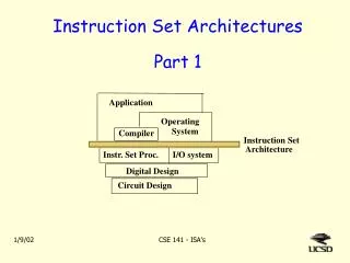
Instruction Set Architectures Chapter 5
Chapter 5 Objectives • Understand the factors involved in instruction set architecture design. • Gain familiarity with memory addressing modes. • Understand the concepts of instruction-level pipelining and its affect upon execution performance.
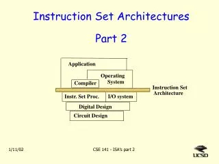
5.1 Introduction • This chapter builds upon the ideas in Chapter 4. • We present a detailed look at different instruction formats, operand types, and memory access methods. • We will see the interrelation between machine organization and instruction formats. • This leads to a deeper understanding of computer architecture in general.
5.2 Instruction Formats Instruction sets are differentiated by the following: • Number of bits per instruction. • Stack-based or register-based. • Number of explicit operands per instruction. • Operand location. • Types of operations. • Type and size of operands.
5.2 Instruction Formats Instruction set architectures are measured according to: • Main memory space occupied by a program. • Instruction complexity. • Instruction length (in bits). • Total number of instruction in the instruction set.
5.2 Instruction Formats In designing an instruction set, consideration is given to: • Instruction length. • Whether short, long, or variable. • Number of operands. • Number of addressable registers. • Memory organization. • Whether byte- or word addressable. • Addressing modes. • Choose any or all: direct, indirect or indexed.
5.2 Instruction Formats • Byte ordering, or endianness, is another major architectural consideration. • If we have a two-byte integer, the integer may be stored so that the least significant byte is followed by the most significant byte or vice versa. • In little endian machines,the least significant byte is followed by the most significant byte. • Big endian machines store the most significant byte first (at the lower address).
5.2 Instruction Formats • As an example, suppose we have the hexadecimal number 12345678. • The big endian and small endian arrangements of the bytes are shown below. Note: This is the internal storage format, usually invisible to the user
5.2 Instruction Formats • Big endian: • Is more natural. • The sign of the number can be determined by looking at the byte at address offset 0. • Strings and integers are stored in the same order. • Little endian: • Makes it easier to place values on non-word boundaries, e.g. odd or even addresses • Conversion from a 32-bit integer to a 16-bit integer does not require any arithmetic.
Standard…What Standard? • Intel (80x86), VAX are little-endian • IBM 370, Motorola 680x0 (Mac), and most RISC systems are big-endian • Makes it problematic to translate data back and forth between say a Mac/PC • Internet is big-endian • Why? Useful control bits in the Most Significant Byte can be processed as the data streams in to avoid processing the rest of the data • Makes writing Internet programs on PC more awkward! • Must convert back and forth
What is an instruction set? • The complete collection of instructions that are understood by a CPU • The physical hardware that is controlled by the instructions is referred to as the Instruction Set Architecture (ISA) • The instruction set is ultimately represented in binary machine code also referred to as object code • Usually represented by assembly codes to human programmer
Elements of an Instruction • Operation code (Op code) • Do this • Source Operand reference(s) • To this • Result Operand reference(s) • Put the answer here • Next Instruction Reference • When you are done, do this instruction next
Where are the operands? • Main memory • CPU register • I/O device • In instruction itself • To specify which register, which memory location, or which I/O device, we’ll need some addressing scheme for each
Instruction Set Design • One important design factor is the number of operands contained in each instruction • Has a significant impact on the word size and complexity of the CPU • E.g. lots of operands generally implies longer word size needed for an instruction • Consider how many operands we need for an ADD instruction • If we want to add the contents of two memory locations together, then we need to be able to handle at least two memory addresses • Where does the result of the add go? We need a third operand to specify the destination • What instruction should be executed next? • Usually the next instruction, but sometimes we might want to jump or branch somewhere else • To specify the next instruction to execute we need a fourth operand • If all of these operands are memory addresses, we need a really long instruction!
Number of Operands • In practice, we won’t really see a four-address instruction. • Too much additional complexity in the CPU • Long instruction word • All operands won’t be used very frequently • Most instructions have one, two, or three operand addresses • The next instruction is obtained by incrementing the program counter, with the exception of branch instructions • Let’s describe a hypothetical set of instructions to carry out the computation for: Y = (A-B) / (C + (D * E))
Three operand instruction • If we had a three operand instruction, we could specify two source operands and a destination to store the result. • Here is a possible sequence of instructions for our equation: Y = (A-B) / (C + (D * E)) • SUB R1, A, B ; Register R1 A-B • MUL R2, D, E ; Register R2 D * E • ADD R2, R2, C ; Register R2 R2 + C • DIV R1, R1, R2 ; Register R1 R1 / R2 • The three address format is fairly convenient because we have the flexibility to dictate where the result of computations should go. Note that after this calculation is done, we haven’t changed the contents of any of our original locations A,B,C,D, or E.
Two operand instruction • How can we cut down the number of operands? • Might want to make the instruction shorter • Typical method is to assign a default destination operand to hold the results of the computation • Result always goes into this operand • Overwrites and old data in that location • Let’s say that the default destination is the first operand in the instruction • First operand might be a register, memory, etc.
Two Operand Instructions • Here is a possible sequence of instructions for our equation (say the operands are registers): Y = (A-B) / (C + (D * E)) • SUB A, B ; Register A A-B • MUL D, E ; Register D D*E • ADD D, C ; Register D D+C • DIV A, D ; Register A A / D • Get same end result as before, but we changed the contents of registers A and D • If we had some later processing that wanted to use the original contents of those registers, we must make a copy of them before performing the computation • MOV R1, A ; Copy A to register R1 • MOV R2, D ; Copy D to register R2 • SUB R1, B ; Register R1 R1-B • MUL R2, E ; Register R2 R2*E • ADD R2, C ; Register R2 R2+C • DIV R1, R2 ; Register R1 R1 / R2 • Now the original registers for A-E remain the same as before, but at the cost of some extra instructions to save the results.
One Operand Instructions • Can use the same idea to get rid of the second operand, leaving only one operand • The second operand is left implicit; e.g. could assume that the second operand will always be in a register such as the Accumulator: Y = (A-B) / (C + (D * E)) • LDA D ; Load ACC with D • MUL E ; Acc Acc * E • ADD C ; Acc Acc + C • STO R1 ; Store Acc to R1 • LDA A ; Acc A • SUB B ; Acc A-B • DIV R1 ; Acc Acc / R1 • Many early computers relied heavily on one-address based instructions, as it makes the CPU much simpler to design. As you can see, it does become somewhat more unwieldy to program.
Zero Operand Instructions • In some cases we can have zero operand instructions • Uses the Stack • Section of memory where we can add and remove items in LIFO order • Last In, First Out • Envision a stack of trays in a cafeteria; the last tray placed on the stack is the first one someone takes out • The stack in the computer behaves the same way, but with data values • PUSH A ; Places A on top of stack • POP A ; Removes value on top of stack and puts result in A • ADD ; Pops top two values off stack, pushes result back on
Stack-Based Instructions Y = (A-B) / (C + (D * E)) • Instruction Stack Contents (top to left) • PUSH B ; B • PUSH A ; B, A • SUB ; (A-B) • PUSH E ; (A-B), E • PUSH D ; (A-B), E, D • MUL ; (A-B), (E*D) • PUSH C ; (A-B), (E*D), C • ADD ; (A-B), (E*D+C) • DIV ; (A-B) / (E*D+C)
How many operands is best? • More operands • More complex (powerful?) instructions • Fewer instructions per program • More registers • Inter-register operations are quicker • Fewer operands • Less complex (powerful?) instructions • More instructions per program • Faster fetch/execution of instructions
Design Tradeoff Decisions • Operation repertoire • How many ops? • What can they do? • How complex are they? • Data types • What types of data should ops perform on? • Registers • Number of registers, what ops on what registers? • Addressing • Mode by which an address is specified (more on this later)
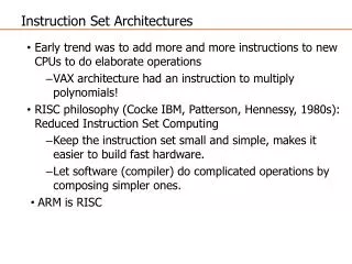
RISC vs. CISC • RISC – Reduced Instruction Set Computer • Advocates fewer and simpler instructions • CPU can be simpler, means each instruction can be executed quickly • Benchmarks: indicate that most programs spend the majority of time doing these simple instructions, so make the common case go fast! • Downside: uncommon case goes slow (e.g., instead of a single SORT instruction, need lots of simple instructions to implement a sort) • Sparc, Motorola, Alpha • CISC – Complex Instruction Set Computer • Advocates many instructions that can perform complex tasks • E.g. SORT instruction • Additional complexity in the CPU • This complexity typically makes ALL instructions slower to execute, not just the complex ones • Fewer instructions needed to write a program using CISC due to richness of instructions available • Intel x86
Instruction Formats • We have seen how instruction length is affected by the number of operands supported by the ISA. • In any instruction set, not all instructions require the same number of operands. • Operations that require no operands, such as HALT, necessarily waste some space when fixed-length instructions are used. • One way to recover some of this space is to use expanding opcodes.
5.2 Instruction Formats Instruction Formats • A system has 16 registers and 4K of memory. • We need 4 bits to access one of the registers. We also need 10 bits for a memory address. • If the system is to have 16-bit instructions, we have two choices for our instructions:
5.2 Instruction Formats Instruction Formats • If we allow the length of the opcode to vary, we could create a very rich instruction set: … … … … How do we tell which address format an instruction is in?
Instruction types Instructions fall into several broad categories that you should be familiar with: • Data movement • Arithmetic • Boolean • Bit manipulation • I/O • Control transfer • Special purpose Can you think of some examples of each of these?
Addressing • Addressing modes specify where an operand is located. • They can specify a constant, a register, or a memory location. • The actual location of an operand is its effective address. • Certain addressing modes allow us to determine the address of an operand dynamically.
Addressing Modes • Addressing refers to how an operand refers to the data we are interested in for a particular instruction • In the Fetch part of the instruction cycle, there are three common ways to handle addressing in the instruction • Immediate Addressing • Direct Addressing • Indirect Addressing
Immediate Addressing • The operand directly contains the value we are interested in working with • E.g. ADD 5 • Means add the number 5 to something • This uses immediate addressing for the value 5 • The two’s complement representation for the number 5 is directly stored in the ADD instruction • Must know value at assembly time
Direct Addressing • The operand contains an address with the data • E.g. ADD 100 • Means to add (Contents of Memory Location 100) to something • Downside: Need to fit entire address in the instruction, may limit address space • E.g. 32 bit word size and 32 bit addresses. Do we have a problem here? • Some solutions: specify offset only, use implied segment • Must know address at assembly time • The address could also be a register • E.g. ADD R5 • Means to add (Contents of Register 5) to something • Upside: Not that many registers, don’t have previous problem
Indirect Addressing • The operand contains an address, and that address contains the address of the data • E.g. Add [100] • Means “The data at memory location 100 is an address. Go to the address stored there and get that data and add it to the Accumulator” • Downside: Requires additional memory access • Upside: Can store a full address at memory location 100 • First address must be fixed at assembly time, but second address can change during runtime! This is very useful for dynamically accessing different addresses in memory (e.g., traversing an array) • Can also do Indirect Addressing with registers • E.g. Add [R3] • Means “The data in register 3 is an address. Go to that address in memory, get the data, and add it to the Accumulator” • Indirect Addressing can be thought of as additional instruction subcycle
Other Addressing Modes • Indexed addressing uses a register (implicitly or explicitly) as an offset, which is added to the address in the operand to determine the effective address of the data. • Based addressing is similar except that a base register is used instead of an index register. • The difference between these two is that an index register holds an offset relative to the address given in the instruction, a base register holds a base address where the address field represents a displacement from this base.
Addressing Example • What value is loaded into the accumulator for each addressing mode? Load 800 Load 800 Load 800 Load R1[800]
Addressing Example • These are the values loaded into the accumulator for each addressing mode. Load R1 using Indirect Addressing?
5.5 Instruction-Level Pipelining • Some CPUs divide the fetch-decode-execute cycle into smaller steps. • These smaller steps can often be executed in parallel to increase throughput. • Such parallel execution is called instruction-level pipelining. • This term is sometimes abbreviated ILP in the literature.
Instruction Prefetch • Simple version of Pipelining – treating the instruction cycle like an assembly line • Fetch accessing main memory • Execution usually does not access main memory • Can fetch next instruction during execution of current instruction • Called instruction prefetch
Improved Performance • But not doubled: • Fetch usually shorter than execution • Prefetch more than one instruction? • Any jump or branch means that prefetched instructions are not the required instructions • Add more stages to improve performance • But more stages can also hurt performance…
Pipelining • Consider the following decomposition for processing the instructions • Fetch instruction – Read into a buffer • Decode instruction – Determine opcode, operands • Calculate operands (i.e. EAs) – Indirect, Register indirect, etc. • Fetch operands – Fetch operands from memory • Execute instructions - Execute • Write result – Store result if applicable • Overlap these operations to make a 6 stage pipeline
Timing of Pipeline • We completed 9 instructions in the time it would take to sequentially complete two instructions! • Assumption for simplicity: • Stages are of equal duration
Instruction-Level Pipelining • The theoretical speedup offered by a pipeline can be determined as follows: Let tp be the time per stage. Each instruction represents a task, T, in the pipeline, with n tasks. The first task (instruction) requires ktp time to complete in a k-stage pipeline. The remaining (n - 1) tasks emerge from the pipeline one per cycle. So the total time to complete the remaining tasks is (n - 1)tp. Thus, to complete n tasks using a k-stage pipeline requires: (ktp) + (n - 1)tp = (k + n - 1)tp.
Instruction-Level Pipelining • If we take the time required to complete n tasks without a pipeline and divide it by the time it takes to complete n tasks using a pipeline, we find: • If we take the limit as n approaches infinity, (k + n - 1) approaches n, which results in a theoretical speedup of:
Instruction-Level Pipelining • Our neat equations take a number of things for granted. • We assume that the pipeline can be kept filled at all times. This is not always the case. Pipeline hazards arise that cause pipeline conflicts and stalls. • Things that can mess up the pipeline • Structural Hazards – Can all stages can be executed in parallel? • What stages might conflict? E.g. access memory • Data Hazards – One instruction might depend on result of a previous instruction • e.g. INC R1 ADD R2,R1 • Control Hazards - Conditional branches break the pipeline • Stuff we fetched in advance is useless if we take the branch
Branch Not Taken Branch Not taken Continue with next instruction as usual
Branch in a Pipeline – Flushed Pipeline Branch Taken (goto Instr 15) Flushed Instructions
Dealing with Branches • Multiple Streams • Prefetch Branch Target • Loop buffer • Branch prediction • Delayed branching
Multiple Streams • Have two pipelines • Prefetch each branch into a separate pipeline • Use appropriate pipeline • Leads to bus & register contention • Still a penalty since it takes some cycles to figure out the branch target and start fetching instructions from there • Multiple branches lead to further pipelines being needed • Would need more than two pipelines then • More expensive circuitry