Download
1 / 42
420 likes | 443 Views
Explore ZDR checks using ice and Bragg regions, self-consistency checks with Z, ZDR, and PHIDP/KDP, reflectivity comparisons, clutter analysis, and ZDR calibration analysis. Learn about estimating ZDR bias from ice/snow, irregular ice/snow analysis, and CP calibration method applications. Dive into self-consistency analysis for Z calibration and examples of good and poor calibration agreements.

E N D
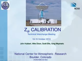
ZDR and Z calibration checksfrom radar echoes, and other methods Mike Dixon, John HubbertScott Ellis, Greg MeymarisNCAR/EOL/RSF NEXRAD Enhancement Project Technical Interchange Meeting Boulder, CO 2016/06/01
Outline ZDR checks using ice and Bragg regions. Self-consistency checks using Z, ZDR and PHIDP/KDP. Reflectivity inter-comparison between SPOL and KDDC. Sun-scan and sun-spike analysis. Clutter analysis for monitoring.
ZDR calibration analysisSPOL during PECAN The top two panels of the following slide summarizes the results of using solar observations and the cross-polar power ratio from clutter to estimate ZDR bias. The third panel shows the measured transmitter power, which is stable throughout the project, varying by only 0.2 dB, in spite of the installation of a replacement trigger amplifier around June 10. The lower panel shows the environmental temperature monitoring for both the site and components in the transmitter container.
Estimating ZDR bias from ICE/SNOW SPOL DBZ PPI SPOL DBZ RHI
Estimating ZDR bias from ICE/SNOW SPOL PID PPI SPOL PID RHI
Select regions for analysis Find ZDR values in these regions. Compute percentile values at say 15%, 20%, 25%. Compare with vertical pointing and CP results. Reflectivity 0 to 30 dBZ SNR 10 to 50 dB RHOHV > 0.98 Max phidp accumulation 10 degrees Max absolute KDP 0.6 deg/km Temperature -5 to -50 C Range 5 km to 120 km Elevation angle 1 to 30 deg 5 consecutive gates of irregular ice/snow Max absolute ZDR 0.75 dB Min number of points in volume: 1000
Estimating ZDR bias from ICE/SNOW SPOL ZDR PPI SPOL ZDR RHI
Estimating ZDR bias from ICE only(region tends to be too small) ZDR in Irregular ICE only
Estimating ZDR bias from ICE/SNOW ZDR in Irregular ICE plus dry snow
Matching up ZDR ice/snow percentile results withvertical pointing and CP method resultsusing daily means
Estimated ZDR bias from ice (red) and Bragg (blue)SPOL during PECANTop: volume-by-volume Bottom: daily means
Temperature dependence of estimated ZDR bias from iceSPOL during PECAN
Time series of ZDR bias estimates from ice (green) and Bragg (blue)along with normalized site temperature (orange) – SPOL PECAN Normalized-temp = (temp – mean) / (sdev * 10)
Time series of ZDR bias estimates from ice (green) and Bragg (blue)along with normalized site temperature (orange) – SPOL PECAN Zoomed on period of interest Normalized-temp = (temp – mean) / (sdev * 10)
From Meymaris presentation, TIM October 2014On using CP ZDR calibration method for KOUNSolar SS values showing diurnal variation
Time series of ZDR bias estimates from ice (green) and Bragg (blue)along with normalized site temperature (orange) – KDDC PECAN Normalized-temp = (temp – mean) / (sdev * 10)
Temperature dependence of estimated ZDR bias from iceKDDC during PECAN
Time series of ZDR bias estimates from ice (green) and Bragg (blue)along with normalized site temperature (orange) – KDDC PECAN Zoomed on period of interest Normalized-temp = (temp – mean) / (sdev * 10)
Time series of ZDR bias estimates from ice (green) and Bragg (blue)along with normalized site temperature (orange) – KGLD PECAN Normalized-temp = (temp – mean) / (sdev * 10) – 0.35
Temperature dependence of estimated ZDR bias from iceKGLD during PECAN
Time series of ZDR bias estimates from ice (green) and Bragg (blue)along with normalized site temperature (orange) – KGLD PECAN Zoomed on period of interest Normalized-temp = (temp – mean) / (sdev * 10) – 0.35
Self-consistency analysis for Z calibration The self-consistency method for checking the calibration of reflectivity is presented in Vivekanandan, et al., 2003. The method is based on the following equation relating Kdp to Z and Zdr: Kdp = 3.32x10⁵ZZdr-2.05 (equation 16 in Vivek. et al., 2003) This equation is applicable to rain regions uncontaminated by ice, hail, graupel, clutter and other non-meteorological echoes. Z and Zdr must be corrected for attenuation. The idea is to find partial rays of radar gates in rain, with some significant change in Phidp, compute Kdp at each gate, integrate over the partial ray to compute estimated Phidp, and then compare that estimate to the measured phidp change over the same gate range.
Ray plot for self-consistency analysisExample of good calibration agreement SNR/DBZ Integrated KDP KDP (red) PID type ZDR vs Zred/blue & smoothed PHIDP The second panel shows good agreement between smoothed PHIDP (green)and estimated PHIDP from integrating estimated KDP (red)
Ray plot for self-consistency analysisExample of poor calibration agreement SNR/DBZ Integrated KDP KDP (red) PID type ZDR vs Zred/blue & smoothed PHIDP The second panel shows poor agreement between smoothed PHIDP (green)and estimated PHIDP from integrating estimated KDP (red)
Self-consistency results for SPOL during PECAN, before corrections.Black: self-consistency results per event. Green: mean for period.Blue: transmitter power measurements.
Self-consistency results for SPOL during PECAN, after corrections.Black: self-consistency results per event. Green: mean for period.Blue: transmitter power measurements.
Self-consistency results for KDDC during PECAN.Black: self-consistency results per event. Green: mean for period.Mean DBZ bias: -0.74 dB
Self-consistency results for KGLD during PECAN.Black: self-consistency results per event. Green: mean for period.Mean DBZ bias: +0.88 dB
Given the close proximity of SPOL tpo KDDC, we cancompare the reflectivity values to check for a bias. The white rectangle is the bounding box for the comparison
Z calibration monitoring – sun scan analysis Using the powers observed during solar scans, and the solar flux observed at the Penticton observatory, we can estimate the receiver gain for each channel. The H receiver gain stays almost constant at 39.0 dB, and the V receiver gain at 39.35 dB, for the entire project. We discovered that the calibration on 2015/06/10 yielded a receiver gain of 38.2 dB for H and 38.7 dB in V, which is 0.8 dB lower than that we have estimated to be the correct receiver gain. As a result reflectivity was 0.8 dB too high for the period from June 10 onwards.
SPOL TRANSMIT / RECEIVE GAINS AND POWERS GRCO GLNAH GWH PRHCO PRVCO HorizLNA CoPolAmp PTH GAH Mitch Switch Tx Ps GAV PTV PRHX PRVX VertLNA XpolAmp GLNAV GRX GWV Measurement plane Switching Rx plane Antenna plane Rx A2D plane Clutter scanning: PRHX/PRVX = (PTV/PTH)(GLNAH/GLNAV) GLNAH/GLNAV = (PRHX/PRVX)(PTV/PTH) Sun scanning: S1 = PRVCO/PRHCO S2 = PRVX / PRHX ZDRM Bias = (PRVX/PRHX)/(S1S2)
Analysis of sun scans to deduce receiver gain.Gain remains constant (within 0.2 dB) through project
Sun-spike analysis for ZDR bias monitoring.From beams that receive solar energy we can estimate the S1S2 ratio.We can also estimate the cross-polar ratio from clutter.Combining these gives us an estimate of ZDR bias (ZDRM)
ZDR calibration using sun spike observations The following slide demonstrates the possibility of using routinely-observed solar spike data for ZDR calibration. The bottom panel shows the S1S2 ratio (from the solar rays) and the cross-polar ratio from clutter. These can be combined to estimate the ZDR bias (ZDRM). The advantage of this method is that it allows us to estimate ZDR bias using routine scanning.
Z and ZDR monitoring – clutter analysis We investigated the option of using clutter field analysis to monitor changes in Z and ZDR over the project. We determined the clutter field as those points at which the clutter return was persistent for over 90% of the time. No weather targets are present for that time fraction. We divided the targets into strong clutter (power -40 to -55 dBm) and weak targets (power -75 to -85 dBm). The -40 dBm max for strong targets was chosen to ensure the receiver was not saturated (it saturates at about -37 dBm). The strong targets are used to analyze clutter returns. The weak targets are used to monitor the occurrence of weather in the clutter domain.
SPOL clutter analysis.We identify persistent clutter targets close to the radar. Median clutter power Clutter frequency (fraction of time)
Targets are divided into two groups – weak and strong.Strong targets are used to monitor Z and ZDR over time.Weak targets are used to detect the presence of weather in the clutter domain. Strong targets (power -55 to -40 dBm) Weak targets (power -85 to -75 dBm)
We analyzed the clutter targets close to the radar over the course of the project.Clutter powers show considerable variability, order 5 dB, so not very helpful for power monitoring.Clutter ZDR seems pretty stable at around -1.3 dB.
Z and ZDR monitoring – clutter analysis We found that the variability in DBZ and ZDR from clutter is not sufficiently stable for calibration purposes. It may be possible to use this technique for monitoring purposes, particularly to warn if the transmitter or receiver changes in a major manner.