Download
1 / 43
440 likes | 528 Views
Learn about equipment calibration against standards, method validation principles, common errors in analysis, and calculation of variance. This text explains calibration curves, linearity, accuracy, precision, and more.

E N D
Calibration Methods Of Equipment & Of Methods
Calibrations • Of equipment • Against known standards • Balances, Pipettes , burets , multi-metres • Specrophotometers • Instruments are compared against international standards
International system of Units (IS) second(time), metre(distance),, kilogram(mass), candela(luminous intensity) mole (amount of substance), Ampere(electric current) and Kelvin(temperature)
Method Validation • Specificity • Linearity • Accuracy • Precision • Range • Limits of Detection and Quantitation
Calibration Methods • Introduction • 1.)Graphs are critical to understanding quantitative relationships • One parameter or observable varies in a predictable manner in relationship to changes in a second parameter 2.) Calibration curve: graph showing the analytical response as a function of the known quantity of analyte • Necessary to interpret response for unknown quantities Time-dependent measurements of drugs and metabolites in urine samples Generally desirable to graph data to generate a straight line
Method Validation - Specificity • How well an analytical method distinguishes the analyte from everything else in the sample. • Baseline separation vs. time time
Errors separate into two broad categories: those originating from the analyst and those originating with the method. The former is an error that is due to poor execution, the latter an error due to an inherent problem with the method. Method validation is designed to minimize and characterize method error. Minimization of analyst error involves education and training. A second way to categorize errors is by whether they are systematic. Systematic errors are predictable and impart a bias to reported results. These errors are usually easy to detect by using blanks, calibration checks, and controls. In a validated method, bias is minimal and well characterized. Random errors are equally positive and negative and are generally small.
Errors • Parallax errors
Distribution of errors • Most measurements will be close to true value. • Larger errors are fewer the larger they are • The average Will be close to true value • This is called Normal distribution
Random errors • Are distributed normally The arithmetic mean is the "standard" average, often simply called the "mean" The standard deviation (SD) quantifies variability. If the data follow a bell-shaped Gaussian distribution, then 68% of the values lie within one SD of the mean (on either side) and 95% of the values lie within two SD of the mean. The SD is expressed in the same units as your data.
Variance Variance is the average squared deviation from the mean of a set of data. It is used to find the standard deviation.
Variance 1. Find the mean of the data. Hint – mean is the average so add up the values and divide by the number of items. • Subtract the mean from each value – the • result is called the deviation from the mean. 3. Square each deviation of the mean. 4. Find the sum of the squares. 5. Divide the total by the number of items.
The variance formula includes the Sigma Notation, , which represents the sum of all the items to the right of Sigma. Variance Formula Mean is represented by and n is the number of items.
Standard Deviation is often denoted by the lowercase Greek letter sigma,. Standard Deviation Standard Deviation shows the variation in data. If the data is close together, the standard deviation will be small. If the data is spread out, the standard deviation will be large.
The bell curve which represents a normal distribution of data shows what standard deviation represents. One standard deviation away from the mean ( ) in either direction on the horizontal axis accounts for around 68 percent of the data. Two standard deviations away from the mean accounts for roughly 95 percent of the data with three standard deviations representing about 99 percent of the data.
Standard Deviation Find the variance. a) Find the mean of the data. b) Subtract the mean from each value. c) Square each deviation of the mean. d) Find the sum of the squares. e) Divide the total by the number of items. Take the square root of the variance.
Standard Deviation Formula The standard deviation formula can be represented using Sigma Notation: Notice the standard deviation formula is the square root of the variance.
Find the variance and standard deviation The math test scores of five students are: 92,88,80,68 and 52. 1) Find the mean: (92+88+80+68+52)/5 = 76. 2) Find the deviation from the mean: 92-76=16 88-76=12 80-76=4 68-76= -8 52-76= -24
Find the variance and standard deviation The math test scores of five students are: 92,88,80,68 and 52. 3) Square the deviation from the mean:
Find the variance and standard deviation The math test scores of five students are: 92,88,80,68 and 52. 4) Find the sum of the squares of the deviation from the mean: 256+144+16+64+576= 1056 5) Divide by the number of data items to find the variance: 1056/5 = 211.2
6) Find the square root of the variance: Find the variance and standard deviation The math test scores of five students are: 92,88,80,68 and 52. Thus the standard deviation of the test scores is 14.53.
Key Areas under the normal Distribution Curve • For normal distributions+ 1 SD ~ 68%+ 2 SD ~ 95%+ 3 SD ~ 99.9%
Calibration Methods • Finding the “Best” Straight Line • 1.)Many analytical methods generate calibration curves that are linear or near linear in nature (i) Equation of Line: where: x = independent variable y = dependent variable m = slope b = y-intercept
Calibration Methods • Finding the “Best” Straight Line • 2.)Determining the Best fit to the Experimental Data (i) Method of Linear Least Squares is used to determine the best values for “m” (slope) and “b” (y-intercept) given a set of x and y values • Minimize vertical deviation between points and line • Use square of the deviations deviation irrespective of sign
Calibration Methods • Finding the “Best” Straight Line • 4.)Goodness of the Fit (i) R2: compares the sums of the variations for the y-values to the best-fit line relative to the variations to a horizontal line. • R2 x 100: percent of the variation of the y-variable that is explained by the variation of the x-variable. • A perfect fit has an R2 = 1; no relationship for R2 ≈ 0 R2 based on these relative differences Summed for each point R2=0.5298 R2=0.9952 Very weak to no relationship Strong direct relationship 53.0% of the y-variation is due to the x-variation What is the other 47% caused by? 99.5% of the y-variation is due to the x-variation
Calibration Methods • Calibration Curve • 1.)Calibration curve: shows a response of an analytical method to known quantities of analyte • Procedure: • Prepare known samples of analyte covering convenient range of concentrations. • Measure the response of the analytical procedure. • Subtract average response of blank (no analyte). • Make graph of corrected response versus concentration. • Determine best straight line.
Calibration Methods • Calibration Curve • 2.)Using a Calibration Curve • Prefer calibration with a linear response - analytical signal proportional to the quantity of analyte • Linear range (LOL) (Limit of linearity ) - analyte concentration range over which the response is proportional to concentration • Dynamic range - concentration range over which there is a measurable response to analyte Additional analyte does not result in an increase in response
Calibration Methods • Calibration Curve • 3.)Impact of “Bad” Data Points • Identification of erroneous data point. - compare points to the best-fit line - compare value to duplicate measures • Omit “bad” points if much larger than average ranges and not reproducible. - “bad” data points can skew the best-fit line and distort the accurate interpretation of data. y=0.091x + 0.11 R2=0.99518 y=0.16x + 0.12 R2=0.53261 Remove “bad” point Improve fit and accuracy of m and b
Calibration Methods • Calibration Curve • 4.)Determining Unknown Values from Calibration Curves • (i)Knowing the values of “m” and “b” allow the value of x to be determined once the experimentally y value is known. (ii) Know the standard deviation of m & b, the uncertainty of the determined x-value can also be calculated
Calibration Methods • Calibration Curve • 5.)Limitations in a Calibration Curve (iv) Limited application of calibration curve to determine an unknown. - Limited to linear range of curve - Limited to range of experimentally determined response for known analyte concentrations Uncertainty increases further from experimental points Unreliable determination of analyte concentration
Calibration Methods • Calibration Curve • 6.)Limitations in a Calibration Curve (v) Detection limit - smallest quantity of an analyte that is significantly different from the blank • where s is standard deviation - need to correct for blank signal - minimum detectable concentration • Where c is concentration • s – standard deviation • m – slope of calibration curve Signal detection limit: Corrected signal: Detection limit:
Calibration Methods • External Standard Addition • 1.)Protocol to Determine the Quantity of an Unknown (i) Known quantities of an analyte are added to the unknown - known and unknown are the same analyte - increase in analytical signal is related to the total quantity of the analyte - requires a linear response to analyte (ii) Very useful for complex mixtures - compensates for matrix effect change in analytical signal caused by anything else than the analyte of interest. (iii) Procedure: (a) place known volume of unknown sample in multiple flasks
Calibration Methods • Standard Addition • 1.)Protocol to Determine the Quantity of an Unknown (iii) Procedure: (b) add different (increasing) volume of known standard to each unknown sample (c)fill each flask to a constant, known volume
Calibration Methods • External Standard Addition • 1.)Protocol to Determine the Quantity of an Unknown (iii) Procedure: (d) Measure an analytical response for each sample - signal is directly proportional to analyte concentration Standard addition equation: Total volume (V):
Calibration Methods • Standard Addition • 1.)Protocol to Determine the Quantity of an Unknown (iii) Procedure: (f)Plot signals as a function of the added known analyte concentration and determine the best-fit line. X-intercept (y=0) yields which is used to calculate from:
Calibration Methods • Internal Standards • 1.)Known amount of a compound, different from analyte, added to the unknown. (i) Signal from unknown analyte is compared against signal from internal standard • Relative signal intensity is proportional to concentration of unknown - Valuable for samples/instruments where response varies between runs - Calibration curves only accurate under conditions curve obtained - relative response between unknown and standard are constant • Widely used in chromatography • Useful if sample is lost prior to analysis Area under curve proportional to concentration of unknown (x) and standard (s)
CALIBRATION OF INSTRUMENTS: CONCENTRATION AND RESPONSE • External Standard: This type of curve is familiar to students as a simple concentration- versus-response plot fit to a linear equation. Standards are prepared in a generic solvent, such as methanol for organics or 1% acid for elemental analyses. Such curves are easy to generate, use, and maintain. For example, if an analysis is to be performed on cocaine, some sample preparation and cleanup is done and the matrix removed or diluted away. In such cases, most interference from the sample matrix is inconsequential, and an external standard is appropriate. External standard curves are also used when internal standard calibration is not feasible, as in the case of atomic absorption spectrometry. • Internal Standard: External standard calibrations can be compromised by complex or variable matrices. In toxicology, blood is one of the more difficult matrices to work with, because it is a thick, viscous liquid containing large and small molecular components, proteins, fats, and many materials subject to degradation. A calibration curve generated in an organic solvent is dissimilar from that generated in the sample matrix, a phenomenon called matrix mismatch. Internal standards provide a reference to which concentrations and responses can be ratioed. The use of an internal standard requires that the instrument system respond to more than one analyte at a time. Furthermore, the internal standard must be carefully selected to mimic the chemical behavior or the analytes.
Example: Calibration standards are prepared from a certified stock solution of cocaine in methanol, which is diluted to make five calibration standards. The laboratory prepares a calibration check in a diluted blood solution using certified standards, and the concentration of the resulting mixture is 125.0 ppb cocaine. When this solution is analyzed with the external- standard curve, the calculated concentration is found to be about half of the known true value. The reason for the discrepancy is related to the matrix, in which unknown interactions mask nearly half of the cocaine present.
Now consider an internal-standard approach An internalstandard of xylocaine is chosen because it is chemically similar to cocaine, but unlikely to be found in typical samples. To prepare the calibration curve, cocaine standards are prepared as before, but 75.0 ppb of xylocaine is included in all calibration solutions.