Tutorial 11 Constrained optimization Lagrange Multipliers KKT Conditions
Tutorial 11 Constrained optimization Lagrange Multipliers KKT Conditions. Constrained Optimization. Constrained optimization problem can be defined as following: Minimize the function, while searching among x , that satisfy the constraints:.


Tutorial 11 Constrained optimization Lagrange Multipliers KKT Conditions
E N D
Presentation Transcript
Tutorial 11Constrained optimization Lagrange MultipliersKKT Conditions
Constrained Optimization Constrained optimization problem can be defined as following: Minimize the function, while searching among x, that satisfy the constraints: For example, consider a problem of minimizing the path f(x) between M and C, so that it touches the constraint h(x)=0. Each ellipse describes the points lying on paths of the same lengths. Again, in the solution the gradient of f(x) is orthogonal to the curve of the constraint. M4CS 2005
Dimensionality Reduction The straightforward method to solve constrained optimization problem is to reduce the number of free variables: If x=(x1,..xn) and there are k constraints h1(x) = 0 ,…, hk(x) = 0, then, the k constraint equations can (sometimes) be solved to reduce the dimensionality of x from n to n-k: M4CS 2005
Surfaces defined by constraint Now we consider the harder case, when dimensionality reduction is impossible. If there are no constraints (k=0), the gradient of f(x) vanishes at the solution x*: In the constrained case, the gradient must be orthogonal to the subspace, defined by the constraints (otherwise a sliding along this subspace will decrease the value f(x), without violating the constraint). M4CS 2005
h2(x)=0 h1(x)=0 λ2∆h2(x) λ1∆h1(x) Explanation The constraints limit the subspace of the solution. Here the solution lies on the intersection of the planes, defined by h1(x)=0 and h2(x)=0. The gradient f(x) must be orthogonal to this subspace (otherwise there is non-zero projection of f(x) along the constraint and the function value can be further decreased). The orthogonal subspace is spanned by λ1 h1(x)+ λ2 h2(x). Thus, at the point of constrained minimum there exist constants λ1 and λ1 , such that: f(x*)= λ1 h1(x*)+ λ2 h2(x*). he more additional constraints are applied, the more restricted is the coordinate of the optimum, but the less restricted is the gradient of the function f(x) (1) M4CS 2005
Lagrange Theorem For the constrained optimization problem There exist a vector , such that the function At the point of constrained minimum Satisfies the equations (1) (2) Motivation for (1) was illustrated on the previous slide, while (2) is an elegant form to re-write constraints . (1) and (2) together can be considered as , where . M4CS 2005
Second derivative As we know from mathematical analysis, zero first derivative is a necessary, but not sufficient condition for the maximum. For example, x2 , x3 , x4 , … all have zero derivative at x=0. Yet, only even powers of x have minimum at 0, while odd powers have a bending point. If the first non-zero derivative is of even order, than the point is extremum, otherwise it is a bending point. Similarly with one dimensional case, the condition (3) is necessary (sufficient if ‘>’) condition of minimum. If the expression (1) is zero or positive semidefinite, the point might be and might not be a minimum, depending on higher order derivatives. In multidimensional case the Taylor terms of order n is a tensor of rank n (slide 5 of Tutorial 11), which analysis for n>2 is beyond the scope of our course. M4CS 2005
Example 1/2 Consider the problem of minimizing f(x)=x+y and constraint that h(x)=x2+y2-1. The minimum is in M4CS 2005
Example 2/2 Now let us check the condition (3,p.7): - this point is minimum • this is not minimum • (actually it is maximum) M4CS 2005
Inequality constraints constraints define a subset of an optimization space. As we have seen earlier, each equality constraints reduces the dimensionality of the optimization space by one. Inequality constraints define geometric limitations without reduction of dimensionality. For example e.g. (x-x0)2 = R2, limits the optimization to the surface of the sphere (n-1 dimensions for n-dimensional space), while (x-x0)2 ≤ R2 limits the search to the internal volume of the sphere (only ‘small’ part of the n-dimensional space, but still n-dimensional). Therefore, the most general case of constrained optimization can be formulated as a set of equality and inequality constraints. M4CS 2005
Inequality constraints: Formal definition Formally, the constrained this general inequality case can be written as (1) One important observation is that at the minimum point the inequality constraints either at the boundary (equality) or void. Really, let assume that at the minimum point x*, for some constraint is in strict inequality: gk(x)<0. This means that any sufficiently small change of x will not violate the constraint the constraint is effectively ‘void’. M4CS 2005
Karush-Kuhn-Tucker conditions Summarizing the above discussion, for the inequality constrained optimization problem (1) we define the Lagrange function as: And the minimum point x* satisfies: 1. 2. 3. Note that µ≥0 in (3). The reason is explained on slide 5, with the difference that inequality constraint will be active only if gradients of the function and the constraint are opposite: M4CS 2005
Karush-Kuhn-Tucker conditions Condition 3 means that each inequality constraint is either active, and in this case it turns into equality constraint of the Lagrange type, or inactive, and in this case it is void and does not constrains the solution. Analysis of the constraints can help to rule out some combinations, however in the general, ‘brute force’ approach the problem with n inequality constraints must be divided into 2^n cases. Each case must be solved independently for a minima, and the obtained solution (if any) must be checked to comply with the constrains: Each constraint, assumed to be loose (valid) must be indeed loose (valid). Then, the lowest minima must be chosen among the received minimums. M4CS 2005
KKT Example 1/5 Consider the problem of minimizing f(x)=4(x-1)2+(y-2)2 with constraints: x + y ≤ 2; x ≥ - 1; y ≥ - 1; Solution: There are 3 inequality constraints, each can be chosen active/ non active yield 8 possible combinations. However, 3 constraints together: x+y=2 & x=-1 & y=-1 has no solution, and combination of any two of them yields a single intersection point. M4CS 2005
KKT Example 2/5 The general case is: We must consider all the combinations of active / non active constraints: (1) (2) (3) (4) (5) (6) (7) (8) Unconstrained: M4CS 2005
KKT Example 3/5 (1) (2) M4CS 2005
KKT Example 4/5 (3) (4) (5) (6) (7) (8) - beyond the range M4CS 2005
KKT Example 5/5 Finally, we compare among the 8 cases we have studied: case (7) resulted was over-constrained and had no solutions, case (8) violated the constraint x+y≤2. Among the cased (1)-(6), it was case (1) , yielding the lowest value of f(x,y). M4CS 2005