Constrained Optimization
Constrained optimization involves maximizing or minimizing functions with restrictions on independent variables. Explore methods such as substitution and Lagrange multipliers in solving economic allocation problems.

Constrained Optimization
E N D
Presentation Transcript
Constrained Optimization So far we have discussed optimizing functions without placing restrictions upon the values that the independent variables can assume. Such problems are often referred to as free maxima and minima or free optima. However, in the real world, often restrictions or constraints are placed upon values of the independent variables. These problems are referred to as constrained optima or constrained optimization.
Constrained Optimization Graphically, the difference between the free optima and the constrained optima can be shown as: Free maximum Constrained maximum constraint
Free maximum Constrained maximum • The free optima occurs at the peak of the surface. • If we specify a specific relationship between variables and (a constraint) then the search for an optimum is restricted to a slice of the surface. The constrained maximum occurs at the peak of the slice. constraint
Constrained Optimization • Since economists deal with the allocation of scarce resources among alternative uses, the concept of constraints or restrictions is important. • There are two approaches to solving constrained optima problems: (i) substitution method (ii) Lagrange multipliers
Substitution Method • Consider a firm producing commodity with the following production function: • Without any constraints, the firm can produce an unlimited quantity by utilizing an unlimited amount of and .
Substitution Method • But suppose the firm has a budget constraint: Let • For simplicity, assume that the maximum amount the firm can spend on these two inputs is $100. • So we have the following constraint:
Substitution Method • Suppose the economic question facing this firm is maximizing production subject to this budget constraint. • The solution via the substitution method is to substitute: • First, write the constraint in terms of :
Substitution Method • Then substitute this value into the production function, such that: • With this substitution, the constrained maxima problem is reduced to a free maxima problem with one independent variable.
Substitution Method • Now apply the usual optimization procedure: (critical value)
Substitution Method • The method of substitution is one way to solve constrained optima problems. This is manageable in some cases. In others, the constraint may be very complicated and substitution becomes complex.
Lagrange Multipliers • The constrained optima problem can be stated as finding the extreme value of subject to . • So Lagrange (a mathematician) formed the augmented function. denotes augmented function will behave like the function if the constraint is followed.
Lagrange Multipliers • Given the augmented function, the first order condition for optimization (where the independent variables are , and λ) is as follows:
Lagrange Multipliers • Using the previous example: note: to be on the budget line
Lagrange Multipliers • Solving these 3 equations simultaneously:
Lagrange Multipliers • Solving these 3 equations simultaneously (cont’d):
Lagrange Multipliers • Solving these 3 equations simultaneously (cont’d):
Lagrange Multipliers • If , then • This solution yields the same answer as the substitution method, i.e., and .
Lagrange Multipliers • Economists prefer using the Lagrange technique over the substitution method, because: easier to handle for most cases and (ii) provides additional information. • Namely for (ii), the value of λ has an economic interpretation. (There is no counterpart to this variable in the substitution method).
Lagrange Multipliers • Given, where C is the level of expenditures (budget = $100 in this example). here the Lagrange multiplier measures the sensitivity of to changes in the constraint (C ).
Lagrange Multipliers • 2nd order conditions Given • 1st order conditions for extremum:
Lagrange Multipliers • 2nd order conditions involve second order partial derivatives expressed in the form of a determinant. • In the constraint case, we will utilize the bordered Hessian – which is the Hessian of the free optima case surrounded by the partial derivatives with respect to the Lagrange multiplier λ.
Lagrange Multipliers • 2nd order partials:
Lagrange Multipliers • 2nd order partials:
Lagrange Multipliers • 2 explanatory variables and 1 constraint is the largest size bordered Hessian we will consider for this class. Note: partials with respect to Lagrange multiplier (λ) form the border
Lagrange Multipliers • So the 2nd order condition is: • Let’s now return to our previous example: • Recall the critical values of , and .
Lagrange Multipliers • What about the 2nd order conditions?
Lagrange Multipliers Find
Lagrange Multipliers Expand by 1st row:
Lagrange Multipliers represents a rel max.