Arid Ecohydrology
Arid Ecohydrology. Ecohydrology Fall 2013. Ecosystem RUE. All terrestrial ecosystems use MAP to create NPP, and are therefore, at some level, water dependent Differential sensitivity to variance in MAP NPP:MAP defines rain use efficiency


Arid Ecohydrology
E N D
Presentation Transcript
Arid Ecohydrology Ecohydrology Fall 2013
Ecosystem RUE • All terrestrial ecosystems use MAP to create NPP, and are therefore, at some level, water dependent • Differential sensitivity to variance in MAP • NPP:MAP defines rain use efficiency • Sensitivity effectively measures the strength of water limitation vis-à-vis nutrient or evolutionary constraints Huxman et al. (2004) - Nature
Convergent RUEmax? • RUEmax generally occurs at low water availability • There is a convergence of RUEmax across all biomes • RUEmax is close to RUEmean for arid sites • RUEmaxis really low compared to RUEmeanfor humid sites
Two Predictions • 1 – NPP will be affected a lot if PPT is driven below the historic minimum • 2 – Removal of other resource limitations will allow RUE to approach RUEmax
Ergo • Water limitation imposes a common constraint on NPP across biomes • Ecosystems have the same RUEmax despite large differences in ppt, physiology, phytogeneticorigin and climate history • Altering resource limitation underscores the relevance of biogeochemistry on NPP (i.e., compared with species)
Inhibited Deep Drainage Over Millenia • In dry areas (<500 mm) there is a nearly ubiquitous pore-water Cl- peak at 5-15 m below grade • Mass balance of Cl yields 10,000-15,000 years of accumulation (without major downward flux event) • Consistent with ~ 1 mm/yr deep drainage Seyfried et al. (2005) - Ecology
But… • Upward water potential gradient • Water is moving out of the soil • Ergo, no downward movement Seyfried et al. (2005) - Ecology
Strong Climatic Control • Cl inventory suggests 7,000-8,000 years of accumulation at a site with 360 mm MAP • Inventory is 1,000 years at 400 mm MAP at nearby site
Ecohydrologic Mechanism • Walvoord et al. (2002) propose a conceptual model to reconcile these attributes • Low water potentials at the base of the root zone were established at the end of the Pleistocene (dramatically increased dryness) • Potentials (< -1 MPa) were maintained continuously during the Holocene • Any deep wetting event would reset the chloride concentrations • Slow upward movement of water above ca. 20 m • Drainage below 20 m of Pleistocene aged water • Simultaneous recharge and upward flux
Vegetation is Essential • Plants are required to impose and maintain the low potentials • Two key attributes: • Deep roots (2-3 m) of sufficient density to capture all downward percolating water • Able to maintain low water potentials at depth continuously • The demand for continuous maintenance has enormous implications for contemporary vegetation management • Clearing vegetation can result in huge fluxes of Cl (and nitrate!) to the deep groundwater
Deep Roots • Root density decreases exponentially with depth, though slower in arid biomes • Max rooting depths ~ 5 m, almost all co-dominant shrubs ~ 1.8 m • Root depths increased with MAP and soil coarseness • Maintaining root potentials demands cavitation avoidance • Geometry of xylem • Soil hydraulic conductance goes to 0 • SW USA co-dominants can withstand cavitation (embolism) from -4 to -9 Mpa (extremely low) • The conceptual model requires sustained -1 MPa at the root zone Sperry et al. (2002) – Functional Ecology
Hydrologic Buffering • Arid lands are hydrologically variable • Model requires constancy • As such, moisture conditions at 2-3 m below grade must be buffered from the surface variability • Water budget suggests that Dd (deep drainage) occurs only when I > (AET + ΔS) • ΔSmax is ~ 350 mm (over 3 m root depth) • Dd occurs only when I is 350 mm > AET • (basically never) • Arid land plants use excess water in wet years • Multiple wet years create rapid vegetation adjustments • Expansion of deep rooted shrubs • Explosion of annuals • As such, the base of the root zone basically are continuously water starved • So why invest in deep roots?
Deep Roots • C expenditure that needs to be net benefit • Existing profile data suggest very little plant available water below 60 cm • 31 yr data record at 2 wk interval • Living roots at 180 cm • Low potentials (< -1.5 Mpa) • Net energy benefit? • Plants may actually be hydrologically subsidizing deep roots to maintain their viability during wet periods • Confers benefits during periods of deep drought Seyfried et al. (2001) – WRR
Implications • Natural deep rooted perennial communities are most frequently replaced with shallow rooted annuals • Grazing, planting • Changes episodic downward fluxes of water and therefore salt, nutrients, hazardous materials • Extremely difficult to reestablish deep rooted vegetation • Adaptive significance of this “ecological inheritance” • Low water potentials, high Cl peaks
What is a “State” • A state is a configuration of a community of organisms that can be described by a set of (dynamic) “state” variables • Biomass, density, species (ages, guilds, abundances), nutrients/organic matter • A “stable state” is a particular configuration that possesses self-reinforcing feedbacks that confer some resilience in the presence of perturbations
Origins of the Idea Stability of populations (constant environment) “If the system of equations describing the transformation of state is nonlinear…there may be multiple stable points with all species present so that local stability does not imply global stability” (Lewontin 1969) Overfishing, invasions, predator removal Stability of ecosystems (variable environment) (Lord) Robert May (1974)
Stable and Non-Stable Equilibria dP/dt = B(P) – D(P) D = a*P + c B = q + K/(1+e-rP) Solve for when dP/dt = 0 or B(P) = D(P)
The Demographic Transition • Introduces ideas: • Equilibria • Disequilibrated systems • Time lags between states • Path dependency?
Demographic Stability – Allee Effects • Per capita birth rates decline at low density • Mate finding, dispersal • Creates two population equilibria • Which is stable? Unstable?
Balls-in-cups • Ball represents an ecosystem state • Cup represents the domain (or basin) of attraction • Remember that there are feedbacks that create “resilience” • Regime shifts occur by: • Perturbation to the variables (i.e., move the ball) • Perturbation to the “fitness landscape” (i.e., change the basin)
Ecosystem Response to Change a. One equilibrium for each environmental condition b. One equilibrium, but rapid rates of change over short span of conditions c. Three equilibria can persist for one state (two stable, one unstable), strong hysteresis (path dependency, temporal lags) in the transition between states
Resilience – A Related Concept • Two aspects of the basin of attraction matter • Width of stability domain [Over what range of conditions/perturbations will the community recover?] • Steepness of the stability domain [How quickly will the system recover?] • Resilience can be used to define both properties • The former is dubbed “ecological resilience” the latter “engineering resilience” • Basically some measure of a systems capacity to buffer the effects of exogenous changes
Hysteresis – A Key Emergent Property • A systems trajectory over time may depend on its current and historical position • Changes in system configuration may delay or even prevent recovery Suding et al. (2005) Trends in Ecology and Evolution
Why Should We Care? • Costly surprises (catastrophic shifts, weak ecosystem responses to management) • Collapse of fishery stocks • Outbreaks of disease • Exotic species invasions • Ecosystem shifts and loss of services • Underscore the complex, contingent (dependent of antecedent conditions) nature of environmental systems • Thresholds imply the need for caution when dealing with complex systems • Climate change, biodiversity loss, stock markets, land use change
Submerged Aquatics Rooted plants little phytoplankton Low turbidity due to: Plant filtration High sediment cohesion limits resuspension due to wind action Algal-dominated Phytoplankton shades SAV High turbidity Reduced filtration Loose, flocculent sediments that can be easily wind-entrained Example: Shallow Lakes
Empirical Evidence • Enrichment of P leads to increased production • Eventually there is sufficient water column P to start to erode the controls exerted by SAV • Catastrophic flip (short time) to phytoplankton dominance • Reductions in P necessary to reverse the process are much larger
Incipient Shifts – Where are the Tipping Points? • Key problem: • It would be nice to know when these are about to happen • Interesting theoretical wrinkles: • Are the conditions for incipient regime shift the same? • Volatility? Stability? • Of sufficient interest to be the subject of an NPR piece
What Kinds of Incipient Shifts? • Multiple settings • Medicine: Onset of asthma and epileptic seizures • Finance: Stock market crashes • Agriculture: Drought-society • Environment: Ocean circulation, fish stocks, rangeland woody cover, boreal climate feedbacks • “Canaries in the coal mine” – predicted catastrophic bifurcations • Volatility/variance • Skewness
Critical Slowing • At critical thresholds, small changes in state or conditions can induce a dramatic shift • That is, the system becomes increasingly “slow” in recovering Scheffer et al. (2009) Nature
How Do You Measure Slowing Down? • Response to experimental perturbations • Measure the rate of return • Impossible to control in large systems, but these are always perturbed • Measure rate at which system fluctuates around the mean • Are the fluctuations autocorrelated? • Are they increasing in time? • Are they changing in their statistical properties? Scheffer et al. (2009) Nature
Autocorrelation, Variance and Skewness Scheffer et al. (2009) Nature Guttal and Jayaprakash 2008 Ecology Letters
Scheffer et al. (2009) Nature
Confronting Theory With Data • Detecting alternative attractors (observational) • Time series shifts • Bimodality in system states (across systems) • Dual relationships to a given control factor Scheffer and Carpenter (2003) TREE
Confronting Theory with Data • Experimentally • Different initial conditions lead to different final states • Disturbance triggered transitions • Path dependency (hysteresis) Scheffer and Carpenter (2003) TREE
Alt. Stable State – Desert Streams • Wetlands used to be a major component of desert streams (Sycamore Creek, AZ) • Reduced to zero over the late 19th and 20th C. • Recently become reestablished with controls on grazing
Basic Mechanism • Wetland plants control sediment dynamics • Density dependent stabilization • Floods and drying are the major hydrologic disturbance in deserts • This makes areas with dense vegetation better able to persist through floods and dry periods, and areas without vegetation less able • Two predicted states – vegetated and gravel bed • Region of global bi-satbility defined by: G – veg growth S – vegetation mortality Ks – channel sediment stability w/o veg Cs – per capita stabilization of sediment rs – scour vegetation mortality V – vegetation Q – flood frequency
Empirical Support • Water and Vegetation cover over time Major Resetting Flood
Vegetation Effects on Vegetation Loss(the biogeomorphic feedback) • Vegetation density affects cover loss • Stream sites self-organize into 1 of 2 modes
Idle Restoration Thoughts • Two strategies for restoration • Change conditions (e.g., reduce P) • Force state (e.g., massive disturbance) • Are there other alternative stable states lurking?
Management and A.S.S. Ecological release Disturbance Changes in herbivory Nutrient enrichment Hydrilla Dominated Native SAV Dominated Physical removal Chemical removal ? Blue-Green Dominated Should massive disturbance be part of the restoration tool-box? Are there states less desirable than the one we’re trying to restore?