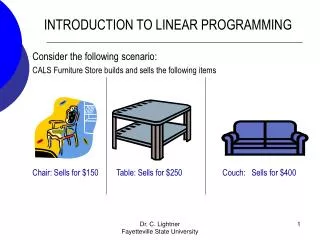
Chapter 7 Introduction to Linear Programming

1. Chapter 7 Introduction to Linear Programming

2. Linear? To get a feel for what linear means let’s think about a simple example. You have $10 to spend and you can buy either M&M’s at 50 cents a bag or Celery at $1 per stalk. Let’s create two columns of numbers where each row will show a combination of Celery and M&M’s you can buy and you will spend the whole $10. The next slide has the information.

3. example The linear idea is related to the idea that when the amount of celery you buy changes by 1 stalk the M&M’s always changes by 2 bags (other examples may not be ratio of 1 to 2). Let’s see on the next screen how we can put this information into a graph, OK :) So, if you buy no celery you can buy 20 bags of M&M’s. If you buy no M&M’s you can have 10 celery stalks. Check the other combinations.

4. example We have to decide which “axis” M&M’s will take and which Celery will take. Let’s say the horizontal axis has been called X1 and the vertical axis X2. I put M&M’s on the vertical axis. In parentheses you see points (X1, X2). This means start at the origin, then go over the value X1 and then go up the value X2. M&M’s X2 (0, 20) (5, 10) Celery X1 All the points are on a straight line. (10, 0) The origin (0, 0)

5. example In the graph we drew, the points on the line imply we spend the whole $10 in the example. If we did not spend the whole $10 we would be inside (south and west) the line. But, with only $10 we can not be outside (north and east) the line. In general, the line represents a limit to what we can get (note the origin is our reference point). In the current example it represents an upper limit. We will see down the road an example where the line might be a lower limit.

6. equation If I = the consumer income in dollars PX1 = the price per unit of Celery PX2 = the price per unit of M&M’s X1 = the amount of celery you buy X2 = the amount of M&M’s you buy, then, in general, the amount you buy is I = (PX1)(X1) + (PX2)(X2) Now, we have I = $10, PX1 = $1 and PX2 = 0.50 so the equation becomes $10 = $1(X1) + $0.05(X2). Since we can have various combinations of X1 and X2, X1 and X2 are left general in the equation. Once we decide on the amount of X1, the amount of X2 we want must satisfy the equation (if we are on the line), and vice versa.

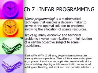
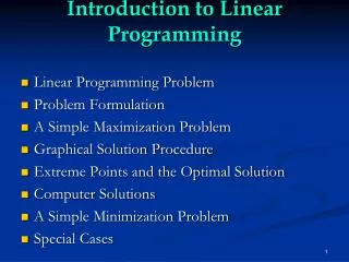
7. Typical linear programming problem Linear programming is a way to handle certain types of optimization problems. By optimize, we typically mean get the most out of something, or in some cases such as with cost, we want to minimize an objective.(you probably would like maximum grade with minimum effort - if not let’s talk) The point is we want to go as far as possible toward reaching some goal. As an example, firms like to maximize profit. This means they would like to get as much profit as possible. The problem is that our actions are constrained or limited. We are constrained in our ability to make profit because we may only have so many machines with which to make product.

8. Product mix problem A basic idea in a problem like this is 1) the company will attempt to maximize profit by selling two or more types of output, 2) The company has only so many inputs to make the output and would like to get as much profit using these inputs, Units of good x1 coming out Decision making inputs Units of good x2 coming out

9. Product mix problem Now, the company has to decide on how much of each type of product to sell. Let’s start with a company with only two goods, good x1 (tables) and good x2 (chairs). Since the objective is to maximize profit we have to know the profit potential for each good. How do we know this? Maybe run regressions, have intuition, whatever, but we need this information. Say the profit per unit on x1 is $7. Then the profit from selling units of x1 equals 7x1. Say the profit for x2 is $5 per unit. So, in general, the profit for the firm is profit = 7x1 + 5x2.

10. Isoprofit lines With the profit in general equal to 7x1 + 5x2, let’s play some scenario analysis, OK? Say we are thinking about profit = $70. We could get this if x1 = 5 and x2 = 7. Or we could get this if x1 = 7 and x2 = 4.2. There are other combinations as well. Once we pick a profit level all the possible x1’s and x2’s that satisfy the equation will be on a straight line. Let’s see this line when profit is $70.

11. Isoprofit lines Note that all these combinations of x1 and x2 would give the same profit. X2 (0, 14) (5, 7) (7, 4.2) X1 (10, 0)

12. Isoprofit lines If we thought of a different profit level we would have a new line, parallel to the first one we looked at. Higher profit levels mean move to lines farther in the northeast. Why don’t we just go to the very farthest out line now and stop? We have constraints in how many units we can make in a given time period. X2 (0, 14) X1 (10, 0)

13. constraints In this product mix problem each table takes 4 hours in the carpentry department and 2 hours in the painting department. Chairs require 3 hours in carpentry and 1 hour in painting. Now we have to know these numbers to do a problem here, and furthermore we have to know the total time available in each department. Say total time in carpentry is 240 hours and painting is 100 hours. Now each department represents a constraint. There is only so much time in each. Tables take 4 hours and chairs only 3 hours in carpentry. We know that the total time to make tables and chairs can not exceed 240 hours in carpentry. It can not be done.

14. Carpentry constraint The time spent on tables is 4x1 and the time spent on chairs is 3x2. The total time spent in carpentry is 4x1 + 3x2 and this amount must be less than or equal to 240 hours. More precisely 4x1 + 3x2 < 240. Note if x1 = 0, x2 = 80 or less, or if x2=0, x1 = 60 or less. There are other points that satisfy the constraint. If we think about the equality part of the equation we could graph all the points that satisfy the equation on a line.

15. Carpentry constraint The line effectively indicates we can make x1 and x2 combinations on the line or to the southwest of the line. You can see now how the constraint limits the profit we can have. WE HAVE ANOTHER CONSTRAINT, TOO! X2 (0, 80) Can’t make this point here because we do not have enough time. X1 (60, 0) Can make this point. Would have time left.

16. Painting constraint The painting constraint turns out to be 2x1 + 1x2 < 100. If x1 = 0, then x2 = 100 or less. If x2 = 0, then x1 = 50 or less. There are other combinations that put us on the line or below the line. Can you find them?

17. Painting constraint I left in the carpentry constraint for reference as the dotted line. The painting constraint is the solid line. We can be on the line or below it. The problem of constraints is that they must all be satisfied! X2 (0, 100) X1 (50, 0)

18. Both constraints Being along this part of the painting constraint means we would violate the carpentry constraint. So the real constraint in this neighborhood is the carpentry constraint. x2 Being along this part of the carpentry constraint means we would violate the painting constraint. So the real constraint in this neighborhood is the painting constraint. x1

19. Both constraints So the real constraint is a combination of the two separate constraints. In the picture you see the company’s Production Possibility neighborhood. Production can not be north and east of the line segments because of the carpentry and painting time constraints. x2 Feasible region x1

20. On the next three slides we will see some general solutions based on different profit amounts for each of the two products. Remember the examples you see are hypothetical.

21. Isoprofit line solution method Remember profit lines will be parallel. x2 Can’t get to p3, Can get p1, but can also get p2. Since we want maximum profit, take p2 and produce only x2 p3 p2 Feasible region p1 x1 Note here profit lines are flatter than the feasible region constraints.

22. Isoprofit line solution method Remember profit lines will be parallel. x2 Can’t get to p3, Can get p1, but can also get p2. Since we want maximum profit, take p2 and produce only x1 p1 p2 p3 Feasible region x1 Note here profit lines are steeper than the feasible region constraints.

23. Isoprofit line solution method x2 Remember profit lines will be parallel. p3 Can’t get to p3, Can get p1, but can also get p2. Since we want maximum profit, take p2 and some x1 and some x2 p2 p1 Feasible region x1 Note here profit lines are not as flat or as steep as the feasible region constraints.