Correlation and Regression
640 likes | 669 Views
Explore the uses and importance of correlation and regression in analyzing the relationships between variables. Learn about assumptions, calculations, significance testing, and nonparametric alternatives. Enhance your statistical skills and avoid common misinterpretations.

Correlation and Regression
E N D
Presentation Transcript
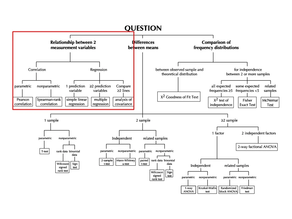
Correlation and Regression • Used when we are interested in the relationship between two variables. • NOTthe differences between means or medians of different groups.
Correlation and Regression • Used when we are interested in the relationship between two variables. • NOTthe differences between means or medians of different groups. The reverse is also true… so in your paper, you should not have written: “There was a correlation between number of pupae and presence of an interspecific competitor.” Rather, the correct way would be: “There was a difference between the mean number of pupae produced between treatments with and without an interspecific competitor.”
Correlation • This is used to: - describe the strength of a relationship between two variables…. This is the “r value” and it can vary from -1.0 to 1.0
Correlation • This is used to: - describe the strength of a relationship between two variables…. This is the “r value” and it can vary from -1.0 to 1.0 - determine the probability that two UNRELATED variables would produce a relationship this strong, just by chance. This is the “p value”.
IF N = 62, then rcrit = 0.250 for p = 0.05, rcrit = 0.325 for p = 0.01
Correlation • Important Note: • Correlation does not imply causation- the variables are related, but one does not cause the second.
Correlation • Important Note: • Correlation does not imply causation - the variables are related, but one does not cause the second. • Often, the variables are both dependent variables in the experiment… such as mean mass of flies and number of offspring. - so it is incorrect to think of one variable as ‘causing’ the other…. As number increases, amount of food per individual declines, and flies grow to a smaller size. Or, as flies grow, small ones need less and so more small ones can survive together than large ones.
Correlation • Parametric test - the Pearson Correlation coefficient. • If the data is normally distributed, then you can use a parametric test to determine the correlation coefficient - the Pearson correlation coefficient.
negative NOTE: no lines drawn through points!
Pearson’s Correlation • Assumptions of the Test • Random sample from the populations • Both variables are approximately normally distributed • Measurement of both variables is on an interval or ratio scale • The relationship between the 2 variables, if it exists, is linear. • Thus, before doing any correlation, plot the relationship to see if its linear!
Pearson’s Correlation • How to calculate the Pearson’s correlation coefficient n = sample size
Testing r • Calculate t using above formula • Compare to tabled t-value with n-2 df • Reject null if calculated value > table value • But SPSS will do all this for you, so you don’t need to!
Example • The heights and arm spans of 10 adult males were measured in cm. Is there a correlation between these two measurements?
Example • Step 2 – Calculate the correlation coefficient - r = 0.932 • Step 3 – Test the significance of the relationship - p = 0.0001
Nonparametric correlation • Spearman’s test • This is the most commonly used test when one of the assumptions of the parametric test cannot be met - usually because it is non-normal, non-linear, or uses ordinal data. • The only assumptions of the Spearman’s r test is that the data is randomly collected and that the scale of measurement is at least ordinal.
Spearman’s test • Like most non-parametric tests, the data are first ranked from smallest to largest • in this case, each column is ranked independently of the other. • Then (1) subtract each rank from the other, (2) square the difference, (3) sum the values, and (4) plug into the following formula to calculate the Spearman correlation coefficient.
Spearman’s test • Calculating Spearman’s correlation coefficient
Testing r • The null hypothesis for a Spearman’s correlation test is also that: • = 0; i.e., H0: = 0; HA: ≠ 0 • When we reject the null hypothesis we can accept the alternative hypothesis that there is a correlation, or relationship, between the two variables.
Testing r • Calculate t using above formula • Compare to tabled t-value with n-2 df • Reject null if calculated value > table value • But SPSS will do all this for you, so you don’t need to!
Example • The mass (in grams) of 13 adult male tuataras and the size of their territories (in square meters) was measured. Are territory size and the size of the adult male tuatara related?
Step 1 – plot the data Note - not very linear
6(60) = rs = 1 - = 0.835 13(168)
Example • Step 2 – Calculate the correlation coefficient • Step 3 – Test the significance of the relationship r = 0.835, p = 0.001 = 5.03
Linear Regression • Here we are testing a causal relationship between the two variables. • We are hypothesizing a functional relationship between the two variables that allows us to predict a value of the dependent variable, y, corresponding to a given value of the independent variable, x.
Regression • Unlike correlation, regression does imply causality • An independent and a dependent variable can be identified in this situation. • This is most often seen in experiments, where you experimentally assign the independent variable, and measure the response as the dependent variable. • Thus, the independent variable is not normally distributed (indeed, it has no variance associated with it!) - as it is usually selected by the investigator.
Linear Regression • For a linear regression, this can be written as: • y = + x (or y = mx + b) • where y = population mean value of y at any value of x • = the population (y) intercept, and • = population slope. • You can use this equation to make predictions - although of course these are usually estimated by sample statistics rather than population parameters.
Linear Regression • Assumptions • 1. The independent variable (X) is fixed and measured without error – no variance. • 2. For any value of the independent variable (X), the dependent variable (Y) is normally distributed, and the population mean of these values of y, y is: • y = + x
Linear Regression • Assumptions • 3. For any value of x, any particular value of y is: • yi = + x + e • Where e, the residual, is the amount by which any observed value of y differs from the mean value of y (analogous to “random error”) • Residuals will follow a standard normal distribution
Linear Regression • Assumptions • 4. The variances of the y variable for all values of x are equal • 5. Observations are independent – each individual is measured only once.
OK Y X
Not OK Y X
Estimating the Regression Function and Line • A regression line always passes through the point: “mean x, mean y”.
Example - Juniper pythonsmeasured single, randomly selected snakes at different temperatures (one snake per temp).
Example Mean x = 10; Mean y = 19.88 How much each value of y (yi) deviates from the mean of y… y – yi • The horizontal line represents a regression line for y when x (temperature) is not considered. • Residuals are very large!
To measure total error, you want to sum the residuals… but they will cancel out… so you must square the differences, then sum. Now we have the TOTAL SUM OF SQUARES (SST) The sum of squares of the residuals is thus: Thus, you see a lot of variance in y when x is not taken into account. How much of the variance in y can be attributed to the relationship with x? Estimating the Regression Function and Line T
Example Mean x = 10; Mean y = 19.88 The “line of best fit” minimizes the residual sum of squares. The best fit line represents a regression line for y when x (temperature) is considered. Now the residuals are very small – in fact, the smallest sum possible.
Estimating the Regression Function and Line • This “line of best fit” minimizes the y sum of squares, and accounts for how x, the independent variable, influences y, the dependent variable. • The difference between the observed values and this “line of best fit” are the residuals – the “error” left over when the relationship is included.
The sum of squares of these regression residuals is now: This is equivalent to the ERROR SS= (SSe); it is the variance “left over” after the realtionship with x has been included. Estimating the Regression Function and Line
Estimating the Regression Function and Line • How do we get this best fit line? • Based on the principles we just went over, you can calculate the slope and the intercept of the best fit line.
Testing the Significance of the Regression Line • In a regression, you test the null hypothesis • Hq: = 0; HA: ≠ 0 • This is done using an ANOVA procedure. • To do this, you calculate sums of squares, their corresponding degrees of freedom, mean squares, and finally an F value (just like an ANOVA!)