Download
1 / 52
520 likes | 695 Views
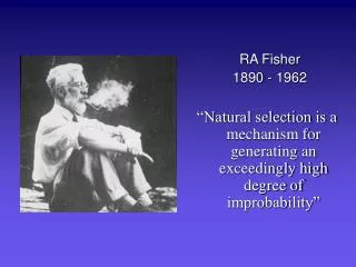
RA Fisher 1890 - 1962. “Natural selection is a mechanism for generating an exceedingly high degree of improbability”. Testing for the Extreme Value Domain of Attraction of Beneficial Fitness Effects. Craig J. Beisel Bioinformatics and Computational Biology Department of Mathematics

E N D
RA Fisher 1890 - 1962 “Natural selection is a mechanism for generating an exceedingly high degree of improbability”
Testing for the Extreme Value Domain of Attraction of Beneficial Fitness Effects Craig J. Beisel Bioinformatics and Computational Biology Department of Mathematics craig@beisel.net www.beisel.net
Concepts Natural SelectionThe differential survival and reproduction of individuals within a population based on hereditary characteristics.
Concepts AdaptationThe adjustment of an organism or population to a new or altered environment through genetic changes brought about by natural selection.
Concepts PhenotypeThe overall attributes of an organism arising due to the interaction of its genotype with the environment.
Concepts GenotypeThe specific genetic makeup of an individual
Concepts FitnessDescribes the ability of a genotype to reproduce. More formally, it is defined as the ratio of the counts of a genotype before and after one generation.
Concepts Fitness LandscapeA function mapping genotype into fitness.
Concepts Fitness DistributionThe distribution of fitness for every possible genotype in a fixed environment. Lethal Moderate High
Mutational Landscape Model John Maynard Smith (1920 – 2004) First remarked that adaptation does not take place in phenotypic space, but in sequence space…
Mutational Landscape Model Gillespie (1983) Given a sequence of nucleotides of length L, There are 4L possible sequences. Each sequence has 3L neighboring sequences which are exactly one point mutation away.
Mutational Landscape Model Additionally, if we assume Strong Selection and Weak Mutation (SSWM) then we can ignore the possibility of clonal interference. Formally 2Ns >>1, Nμ<1 Therefore new mutants will fix (or not) in the population before the next mutant arises. Also, double mutants and neutral/deleterious mutations can be ignored.
Mutational Landscape Model Consider a sequence in an environment where it is currently the most fit. A small change occurs in the environment which shifts it to be the ith most fit sequence among its one-step mutant neighbors where i is small.
Mutational Landscape Model There are then i-1 more fit sequences which the population could move to. Notice that the fitnesses of these sequences are in the tail of the fitness distribution.
Mutational Landscape Model We would like to find the probability of the population fixing mutant j when starting with sequence i. Since we are dealing with only the tail of the fitness distribution we can apply EVT.
Orr’s One Step Model Assumptions The fitness distribution is in the Gumbel domain of attraction and therefore the fitnesses of the i-1 more fit one-step mutants can be considered to be drawn from an ‘exponential’ distribution by GPD. This will allow a result which is independent of the underlying fitness distribution.
Orr’s One Step Model Lemma Let X1,…, Xn be iid observations where Xi~Exp and X(1),…,X(n) be their corresponding order statistics. Then the spacings defined ΔXi = X(i-1) – X(i) are distributed exponential and E(ΔXi)= ΔX1 / i Sukhatme (1937)
Orr’s One Step Model Sincej 2sj (Haldane 1927)
Orr’s One Step Model Taking the expected value…
Orr’s One Step Model Notice, we have an expression for the expected transition probability which is independent of the fitness of the individual sequences and depends only on i and j.
Orr’s One Step Model Can this model be validated empirically?
Orr’s One Step Model Experimental Evolution Natural Isolate ID11 ~3% differ from G4 Microviridae Host - E. Coli 5577 bp
Orr’s One Step Model 20 one-step walks 9 observed mutations Rokyta et al (2005)
Orr’s One Step Model Concluded Orr’s transition probabilities did not explain data as well as Wahl model even after correcting the model for mutation bias.
Orr’s One Step Model Where did Orr go wrong? Perhaps, the tail of the fitness distribution is not in the Gumbel domain of attraction and therefore not exponentially distributed?
Extreme Value Theory Extreme Value Theory Field of statistical theory which attempts to describe the distribution of extreme values (maxima and minima) of a sample from a given probability distribution.
Extreme Value Theory Notice that extreme values of a sample generally fall in the tail of the underlying probability distribution. For example the maximum of a sample of size 10 from a standard normal distribution…
Extreme Value Theory Since the tail is all that must be considered, many results of extreme value theory are independent of the underlying probability distribution. In fact, EVT shows almost all probability distributions can be classified into three groups by their tail behavior.
Extreme Value Theory These three types are… Gumbel Most Common Distributions Exponential, Normal, Gamma, etc. Weibull Finite Tail distributions Fréchet Heavy Tail Distributions Cauchy
Extreme Value Theory EVT allows all three types of tail behavior to be described by the Generalized Pareto Distribution (GPD) tau – scale kappa-shape
Extreme Value Theory EVT allows all three types of tail behavior to be described by the Generalized Pareto Distribution (GPD)
Extreme Value Theory The GPD not only provides the natural alternative distribution for testing against the exponential in this context, the null model of k=0 is nested which allows the application of Maximum Likelihood and Likelihood Ratio Testing.
Maximum Likelihood and LRT Log-Likelihood for the GPD is given…
Maximum Likelihood and LRT Distribution of the LRT test statistic? Although a common approximation is to assume Chi-squared with one degree of freedom, this does not appear to be the case here. Distribution of the test statistic was calculated using parametric bootstrap.
Maximum Likelihood and LRT Power Probability of rejecting the null when the alternative is true. 1-P(Type II error) Can we hope to reject the null with a given data set?
Maximum Likelihood and LRT Sensitivity Analysis Determine the inflation of the Type I error rate under violations of the null. If null is rejected, what is the chance that rejection was due to inflation of alpha due to violations in the assumptions of the null hypothesis?
Maximum Likelihood and LRT • Violations of the Null Assumptions • Small effect mutations have low probability of fixation and therefore may not be observed. • Observations include measurement error which may be normal or log-normal.
Maximum Likelihood and LRT GPD is stable to shifts of threshold, analyze data relative to the smallest observed!
Maximum Likelihood and LRT If measurement error is not considered and our test rejects it is likely that we are safe in our conclusion assuming error is small. In the event that we fail to reject, it is likely due to the loss of power encountered when operating under a false null hypothesis. In this case, we must reanalyze our data incorporating measurement error.
Maximum Likelihood and LRT The likelihood equation of normal or lognormal measurement error conditional on the GPD has no closed form ;(
Maximum Likelihood and LRT Standard optimization procedures fail to converge…
Metropolis-Hastings and Bayesian Methods MH Algorithm Given X(t) 1. Generate Y(t) ~ g(y-x(t)) 2. Take X(t) = Y(t) with probability min(1,f(Y(t))/f(X(t))) X(t) otherwise If g(z) is normal (symmetric) then convergence to posterior is assured
Metropolis-Hastings and Bayesian Methods tau=1, kappa=-2, sigma=.1 mean=-1.64 95%CI=(-.826,-2.70)
Metropolis-Hastings and Bayesian Methods tau=1, kappa=-2, sigma=.1 mean=.893 95%CI=(.509,1.41)
Metropolis-Hastings and Bayesian Methods tau=1, kappa=-2, sigma=.1 mean=-1.818 CI=(-1.47,-2.23)
Metropolis-Hastings and Bayesian Methods tau=1, kappa=-2, sigma=.1 mean=.083 95%CI=(.034,.160)