Download
1 / 28
290 likes | 398 Views
Explore the Flux-Transport Dynamo model for simulating and forecasting solar cycles, utilizing observational signatures and dynamo processes.

E N D
SIMULATING AND PREDICTING SOLAR CYCLES USING A FLUX-TRANSPORT DYNAMO Mausumi DikpatiHigh Altitude Observatory, NCAR Principal collaborator: Peter Gilman (HAO/NCAR) Other collaborators: C.N. Arge (AFGL), P. Charbonneau (Montreal), G. de Toma (HAO/NCAR), D.H. Hathaway (NASA/MSFC), K.B. MacGregor (HAO/NCAR), M. Rempel (HAO/NCAR), O.R.White (HAO/NCAR)
Random vs. persistent, cyclic features active longitudes mixed-polarity turbulent fields Courtesy: T. Berger butterfly diagram, polar reversal Courtesy: G. de Toma Courtesy: D.H. Hathaway
What is a dynamo? A dynamo is a process by which the magnetic field in an electrically conducting fluid is maintained against Ohmic dissipation In astrophysical object, there can always be a dynamo whenever the plasma consists of seed magnetic fields and flow fields
Observational signature forrandom evolution of magnetic fields Courtesy: P. Sutterlin, Dutch Open Telescope Team, SUI
Observational signature for systematic, cyclic evolution of solar magnetic fields Courtesy: D.H. Hathaway Many evidences for coexistence of small-scale and large-scale dynamos
Large-scale dynamo processes < (i) Generation of toroidal (azimuthal) field by shearing a pre-existing poloidal field (component in meridional plane) by differential rotation (Ω-effect ) (ii) Re-generation of poloidal field by lifting and twisting a toroidal flux tube by helical turbulence (α-effect) (iii) Flux transport by meridional circulation = FLUX-TRANSPORT DYNAMO
A possible α-effect arising from decay of tilted bipolar active regions Babcock 1961, ApJ, 133, 572
Mathematical Formulation Under MHD approximation (i.e. electromagnetic variations are nonrelativistic), Maxwell’s equations + generalized Ohm’s law lead to induction equation : (1) Applying mean-field theory to (1), we obtain the dynamo equation as, (2) Diffusion (turbulent + molecular) Differential rotation and meridional circulation Displacing and twisting effect by kinetic helicity
Evolution of Magnetic FieldsIn a Babcock-Leighton Flux-Transport Dynamo Dynamo cycle period ( T ) primarily governed by meridional flow speed Dikpati & Charbonneau 1999, ApJ, 518, 508
Analogy with ocean conveyor belt Broecker 1991
Calibrated Flux-transport Dynamo Model Flows derived from observations Magnetic diffusivity used N-Pole Red: α -effect location Green: rotation contours Blue: meridional flow S-Pole Near-surface diffusivity same as used by Wang, Shelley & Lean, 2002; Schrijver 2002 in their surface flux-transport models.
Validity test of calibration Contours: toroidal fields at CZ base Gray-shades: surface radial fields Observed NSO map of longitude-averaged photospheric fields (Dikpati, de Toma, Gilman, Arge & White, 2004, ApJ, 601, 1136)
Precursor methods Schatten 2005, GRL
Flux-transport Dynamo-based Prediction Scheme We postulate that “magnetic persistence”, or the duration of the Sun’s “memory” of its own magnetic field, is controlled by meridional circulation. <
Construction of surface poloidal source from observations (contd.) Original data (from Hathaway) Period adjusted to average cycle Assumed pattern extending beyond present
Three techniques for treating surface poloidal source in simulating and forecasting cycles Forecasted quantity : integrated toroidal magnetic flux at the bottom in latitude range of 0 to 45 degree (which is the sunspot-producing field) 1) Continuously update of observed surface source including cycle predicted (a form of 2D data assimilation) 2) Switch off observed surface source for cycle to be predicted 3) Substitute theoretical surface source, derived from dynamo-generated toroidal field at the bottom, for observed surface source We use these three techniques in succession to simulate and forecast
Simulating relative peaks of cycles 12 through 24 (model fed by surface poloidal source continuously) Observed cycles • We reproduce the sequence of peaks of cycles 16 through 23 • We predict cycle 24 will be 30-50% bigger than cycle 23 • We obtain similar results for diffusivities between and (Dikpati, de Toma & Gilman, 2006, GRL, in press)
How does the model work? Red and blue contours are poloidal field lines in the plane of the board; red (blue) denotes clockwise (counterclockwise) field directions Color shades denote toroidal field strengths; orange/red denotes positive (into board) fields, green/blue negative Latitudinal component of poloidal fields near the bottom is primary source of new toroidal fields
How does the model work? (Contd.) Toroidal B Latitudinal B Latitudinal fields in the conveyor belt from past 3 cycles combine near the bottom to form the source of new cycle toroidal field. Mechanism is shearing by latitudinal differential rotation. (Dikpati & Gilman, 2006, ApJ, in preparation)
Comparison of effects of zero and continuously updated surface sources on predicted cycles Continuous poloidal source updating Zero poloidal source Peak of cycle 20 is the same as when continually update surface poloidal source; but cycle 21 is nearly zero. This is true for diffusivities up to about Above that, dynamo is increasingly diffusion-dominated, and loses memory of past cycles Can we forecast beyond one cycle ahead?
Surface poloidal source constructed from the predicted bottom toroidal field; BL flux-transport dynamo in self-excited mode
Skill tests Zero poloidal source for predicted cycles Babcock-Leighton poloidal source (from bottom toroidal field) for predicted cycles
Summary and future directions • Flux-transport dynamo with input of observed surface magnetic flux displays high skill in forecasting peak of the next solar cycle, as well as significant skill for 2 cycles ahead • We will do specific forecast for cycle 25 in the near future • Test forecast-model back to cycle 1 • Simulate and forecast differences between N and S hemispheres • Go beyond longitude-averaged solar cycle features, e.g., simulate and predict ‘active longitudes’ (in progress – supported by opportunity fund)