Classical Discrimination: Understanding Classification Methods
700 likes | 719 Views
Explore classical discrimination methods like Fisher Linear Discrimination (FLD) and Gaussian Likelihood Ratio (GLR) for classification problems. Learn the basics, derivations, and graphical representations to understand and apply these techniques effectively.

Classical Discrimination: Understanding Classification Methods
E N D
Presentation Transcript
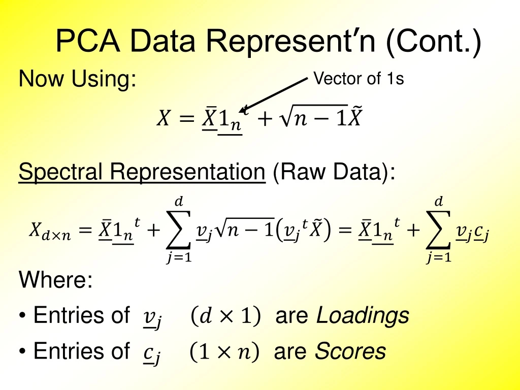
PCA Data Represent’n (Cont.) Vector of 1s • Now Using: • Spectral Representation (Raw Data): • Where: • Entries of are Loadings • Entries of are Scores
PCA Data Represent’n (Cont.) • Reduced Rank Representation: • Reconstruct Using Only Terms • (Assuming Decreasing Eigenvalues)
Return to Big Picture Main statistical goals of OODA: • Understanding population structure • Low dim’al Projections, PCA … • Classification (i. e. Discrimination) • Understanding 2+ populations • Time Series of Data Objects • Chemical Spectra, Mortality Data • “Vertical Integration” of Data Types
Classification - Discrimination Background: Two Class (Binary) version: Using “training data” from Class +1 and Class -1 Develop a “rule” for assigning new data to a Class Canonical Example: Disease Diagnosis • New Patients are “Healthy” or “Ill” • Determine based on measurements
Classification Basics For Simple Toy Example: Project On MD & split at center
Classification Basics Mean Difference for slanted clouds: A little better? Still misses right dir’n Want to account for covariance
Classification Basics Better Solution: Fisher Linear Discrimination Gets the right dir’n How does it work?
Fisher Linear Discrimination Simple way to find “correct cov. adjustment”: Individually transform subpopulations so “spherical” about their means For = +,- define
Fisher Linear Discrimination In Transformed Space, Separating Hyperplane has: Transformed Normal Vector: Transformed Intercept: Separating Hyperplane Has Eqn.
Fisher Linear Discrimination Thus discrimination rule is: Classify to Class +1 when: where: i.e. Same Inner Product Of Center Point Inner Product of New Data Point & Transf’d Direction
Classical Discrimination Above derivation of FLD was: • Nonstandard • Not in any textbooks(?) • Nonparametric (don’t need Gaussian data) • I.e. Used no probability distributions • More Machine Learning than Statistics (but careful about HDLSS case)
Classical Discrimination FLD Likelihood View Assume: Class distributions are multivariate for = +,- • strong distributional assumption + common covariance (Within Class)
Classical Discrimination FLD Likelihood View (cont.) At a location , the likelihood ratio, for choosing between Class +1 and Class -1, is: where is the Gaussian density with covariance
Classical Discrimination FLD Likelihood View (cont.) Simplifying, using the Gaussian density: Gives (critically using common covariances): =
Classical Discrimination FLD Likelihood View (cont.) But: for
Classical Discrimination FLD Likelihood View (cont.) But: so: Note: same terms subtract off
Classical Discrimination FLD Likelihood View (cont.) But: so: Note: cross terms have ± cancellation Seen in Above Nonparametric Derivation Similar To AboveCenter
Classical Discrimination FLD Likelihood View (cont.) But: so: Thus when i.e.
Classical Discrimination FLD Likelihood View (cont.) Replacing , and by maximum likelihood estimates: , and Gives the likelihood ratio discrimination rule: Choose Class +1, when Same as above, so: FLD can be viewed as Likelihood Ratio Rule
Classical Discrimination FLD Generalization I Gaussian Likelihood Ratio Discrimination (a. k. a. “nonlinear discriminant analysis”) Idea: Assume class distributions are Differentcovariances! Likelihood Ratio rule is straightf’dnum’l calc. (thus can easily implement, and do discrim’n)
Classical Discrimination Gaussian Likelihood Ratio Discrim’n (cont.) No longer have separ’g hyperplanerepr’n (instead regions determined by quadratics) (fairly complicated case-wise calculations) Graphical display: for grid of test points, color as: Yellow if assigned to Class +1 Cyan if assigned to Class -1 (intensity is strength of assignment)
Classical Discrimination Graphical Display of Classifiers Use Yellow for Grid Points Assigned to Plus Class Use Cyan for Grid Points Assigned to Minus Class
Classical Discrimination FLD for Tilted Point Clouds – Works well
Classical Discrimination GLR for Tilted Point Clouds – Works well
Classical Discrimination FLD for Donut – Poor, no plane can work
Classical Discrimination GLR for Donut – Works well (good quadratic) (Even though data not Gaussian)
Classical Discrimination FLD for X – Poor, no plane can work
Classical Discrimination GLR for X – Better, but not great
Classical Discrimination Summary of FLD vs. GLR: • Tilted Point Clouds Data • FLD good • GLR good • Donut Data • FLD bad • GLR good • X Data • FLD bad • GLR OK, not great Classical Conclusion: GLR generally better (will see a different answer for HDLSS data)
Classical Discrimination FLD Generalization II (Gen. I was GLR) Different prior probabilities Main idea: Give different weights to 2 classes • I.e. assume not a priori equally likely Canonical Example: Rare Disease Testing (Often Train on Mostly Rare Cases)
Classical Discrimination FLD Generalization II (Gen. I was GLR) Different prior probabilities Main idea: Give different weights to 2 classes • I.e. assume not a priori equally likely • Development is “straightforward” • Modified likelihood • Change intercept in FLD • Won’t explore further here
Classical Discrimination FLD Generalization III Principal Discriminant Analysis Also Called: Multiple Discriminant Analysis Duda, et al. (2001) Canonical Variate Analysis Mardia, et al. (1979)
Classical Discrimination FLD Generalization III Principal Discriminant Analysis • Idea: FLD-like approach to > 2 classes • Assumption: Class covariance matrices are the same (similar) (but not Gaussian, same situation as for FLD) • Main idea: Quantify “location of classes” by their means
Classical Discrimination Principal Discriminant Analysis (cont.) Simple way to find “interesting directions” among the means: PCA on set of means (Think Analog of Mean Difference)
Classical Discrimination Principal Discriminant Analysis (cont.) Simple way to find “interesting directions” among the means: PCA on set of means i.e. Eigen-analysis of “between class covariance matrix” Where Aside: can show: overall Mean of Means
Classical Discrimination Principal Discriminant Analysis (cont.) But PCA only works like Mean Difference, Expect can improve by taking covariance into account. (Recall Improvement of FLD over MD)
Classical Discrimination Principal Discriminant Analysis (cont.) But PCA only works like Mean Difference, Expect can improve by taking covariance into account. Blind application of above ideas suggests eigen-analysis of:
Classical Discrimination Principal Discriminant Analysis (cont.) There are: • smarter ways to compute (“generalized eigenvalue”) • other representations (this solves optimization prob’s) Special case: 2 classes, reduces to standard FLD Good reference for more: Section 3.8 of: Duda et al. (2001)
Classical Discrimination Summary of Classical Ideas: • Among “Simple Methods” • MD and FLD sometimes similar • Sometimes FLD better • So FLD is preferred • Among Complicated Methods • GLR is best • So always use that? • Caution: • Story changes for HDLSS settings
HDLSS Discrimination Main HDLSS issues: • Sample Size, < Dimension, • Singular covariance matrix • So can’t use matrix inverse • I.e. can’t standardize (sphere) the data (requires root inverse covariance) • Can’t do classical multivariate analysis
HDLSS Discrimination Main HDLSS issues: • Can’t do classical multivariate analysis • Key Idea: Standardize • Subtract Sample Mean • Sphere the Data (i.e. Multiply by ) • And use dist’n for statistical inference
HDLSS Discrimination An approach to non-invertible covariances: • Replace by generalized inverses • Sometimes called pseudo inverses • Note: there are several • Here use Moore Penrose inverse • As used by Matlab (pinv.m) • Often provides useful results (but not always)
HDLSS Discrimination Application of Generalized Inverse to FLD: Direction (Normal) Vector: Intercept:
HDLSS Discrimination Application of Generalized Inverse to FLD: Direction (Normal) Vector: Intercept: Have replaced by
HDLSS Discrimination Toy Example: Increasing Dimension data vectors: • Entry 1: Class +1: Class –1: • Other Entries: • All Entries Independent Look through dimensions,
HDLSS Discrimination Project on Optimal Direction Increasing Dimension Example Project on FLD Direction Project on Both
HDLSS Discrimination Same Projections on Optimal Direction Add a 2nd Dimension ( noise) Axes Here Are Same As Directions Here Now See 2 Dimensions
HDLSS Discrimination Add a 3rd Dimension (noise) Project on 2-d subspace generated by optimal dir’n & by FLD dir’n
HDLSS Discrimination Movie Through Increasing Dimensions
HDLSS Discrimination FLD in Increasing Dimensions: • Low dimensions (d = 2-9): • Visually good separation • Small angle between FLD and Optimal • Good generalizability • Medium Dimensions (d = 10-26): • Visual separation too good?!? • Larger angle between FLD and Optimal • Worse generalizability • Feel effect of sampling noise


