Download
1 / 96
980 likes | 1.1k Views
Learn about the history and paradigms of statistical physics in complex networks, from fractals to cellular automata. Discover the importance of studying complex network topology and its applications in various fields. Dive into biomolecular networks, technological networks, and network modeling principles.

E N D
Statistical physics of complex networks Sergei Maslov Brookhaven National Laboratory
Short history: complex systems before & after networks • Statistical physics of complex systems was active in 80’s-90’s (following the chaos boom of 70’s) • Fractals (Mandelbrot and many others) • Self-Organized Criticality (Per Bak and co-authors) sandpiles granular systems • Complex==multiple time and length scales (e.g. avalanches) Cult of power-laws • Cellular automata (mostly in real space+time) • Examples: • earthquakes • disordered moving interfaces • (co)-evolution of species • agent-based modeling (“ants”) • By the end of 90’s breakup of the community and specialization • Biology • Economics and finance • Internet • Social sciences
Networks in complex systems • Complex systems • Large number of components interacting with each other • All components and/or interactions are different from each other (unlike in traditional physics where 1023 electrons are all the same!) • Paradigms: • 104 types of proteins in an organism, • 106 routers in the Internet • 109 web pages in the WWW • 1011 neurons in a human brain • The simplest property: who interacts with whom? can be visualized as a network • Complex networks are just a backbone for complex dynamical processes
Why study the topology of complex networks? • Lots of easily available data: that’s where the state of the art information is (at least in biology) • Large networks may contain information about basic design principles and/or evolutionary history of the complex system • This is similar to paleontology: learning about an animal from its backbone
Protein binding networks Baker’s yeast S. cerevisiae(only nuclear proteins shown) Nematode worm C. elegans
Transcription regulatory networks Single-celled eukaryote:S. cerevisiae Bacterium:E. coli
GENOME protein-gene interactions PROTEOME protein-protein interactions METABOLISM bio-chemical reactions slide after Reka Albert
Sea urchin embryonic development (endomesoderm up to 30 hours) by Davidson’s lab
Sexual contacts: M. E. J. Newman, The structure and function of complex networks, SIAM Review 45, 167-256 (2003).
High school dating: Data drawn from Peter S. Bearman, James Moody, and Katherine Stovel visualized by Mark Newman
Webpages connected by hyperlinks on the AT&T website circa 1996 visualized by Mark Newman Citation networks are similar to the WWW but time-ordered
Internet as measured by Hal Burch and Bill Cheswick's Internet Mapping Project.
transportation networks: railway maps Tokyo rail map
Lecture 1: General introduction into networks • Node degrees, its distribution, and correlations • Simple models • preferential attachment and Simon model • Growth model for protein families • Percolation transition on networks • Clustering coefficient • Lectures 2-3: Biomolecular (mostly protein) networks • Regulatory and signaling networks • How many regulators? Bureaucratic collapse • Network motifs in directed (e.g. regulatory) networks • Protein binding networks • Broad degree distributions in protein binding networks and possible explanations • Evolutionary (duplication-divergence) • Biophysical (stickiness) • Functional • Beyond degree distributions: How it all is wired together? Correlations in degrees • Randomization of networks • Law of Mass Action and propagation of perturbations • Lecture 4: Technological and information networks • Diffusion and modules in the Internet, WWW, and scientific citations • Predicting opinions of customers on products (e.g. movies) using knowledge networks
Degree (or connectivity) of a node – the # of neighbors Degree K=2 Degree K=4
Directed networks havein- and out-degrees In-degree Kin=2 Out-degree Kout=5
Poisson distribution Degree distribution in a random network • Randomly throw E edges among N nodes • Solomonoff, Rapaport, Bull. Math. Biophysics (1951)Erdos-Renyi (1960) • Degree distribution – Binominal Poisson • K~ with no hubs(fast decay of N(K))
Degree distribution in real protein binding network • Histogram N(K) is broad: most nodes have low degree ~ 1, few nodes – high degree ~100 • Can be approximately fitted with N(K)~K- functionalformwith ~=2.5
3 1 2 Basic BA-model • Very simple algorithm to implement • start with an initial set of m0 fully connected nodes • e.g. m0 = 3 • now add new vertices one by one, each one with exactly m edges • each new edge connects to an existing vertex in proportion to the number of edges that vertex already has → preferential attachment • easiest if you keep track of edge endpoints in one large array and select an element from this array at random • the probability of selecting any one vertex will be proportional to the number of times it appears in the array – which corresponds to its degree 1 1 2 2 2 3 3 4 5 6 6 7 8 ….
3 1 1 2 2 3 3 3 4 1 1 1 1 1 2 2 2 3 3 34 4 2 2 2 5 3 4 1 1 2 2 2 3 3 3 3 4 4 4 5 5 generating BA graphs – cont’d • To start, each vertex has an equal number of edges (2) • the probability of choosing any vertex is 1/3 • We add a new vertex, and it will have m edges, here take m=2 • draw 2 random elements from the array – suppose they are 2 and 3 • Now the probabilities of selecting 1,2,3,or 4 are 1/5, 3/10, 3/10, 1/5 • Add a new vertex, draw a vertex for it to connect from the array • etc.
The tale of linear vs exponential growth • Linear growth: Barabasi-Albert model with =3 is a version of the Simon’s word usage model: =2+ • dnk/dt=(k-1)nk-1/(t+t)-knk/(t+t) • Exponential growth: Protein duplication-deletion model: =2+/(dup-del) • dnk/dt=dup (k-1)nk-1- (dup+del )knk++del (k+1)nk+1; NF=knk also grows exponentially: dNF/dt= NG= kknk
Preferential attachment with fitness • Bianconi-Barabasi (2001) • Attractiveness of a node to new edges is given by fiki/rfrkr • For uniform (f): Pk ~ k-(1+C*)/ln(k), where C*=1.255 • Generally C depends on (f) • Some (f) result in “Bose-Einstein condensation” in which super-hubs emerge
Why should we care? • The most important property of a network. It quantifies how broken-up is a network • Below the percolation threshold: many small components • At the percolation threshold: scale-free distribution of component sizes: P(S)=S-2.5 • Above the percolation threshold: giant connected component and a few small ones? • Determines the propagation of perturbations which affect neighbors with probability p (e.g. infections)
Naïve (and wrong) argument • An average node has <K>first neighbors, <K><K-1>second neighbors, <K><K-1><K-1>third neighbors • We neglect overlap between e.g. second and first neighbors: in random networks a small effect ~1/N • If <K-1> 1 a single node is connected to a finite fraction of all nodes in the network
Where is it wrong? • Probability to arrive at a node with K neighbors is proportional to K! • All averages have to be modified <F(K)> <F(K) K>/<K> • The right answer: <K(K-1)>/<K> 1a perturbation would spread • In directed networks it is <KinKout>/<Kin> 1 • Correlations between degrees of neighbors and an abnormally large number of triangles (clustering) would affect the answer
How many clusters? • If <K(K-1)>/<K> <<1 there are only small clusters • If<K(K-1)>/<K> 1cluster sizes S have a scale-free distribution: P(S)~S-2.5. • If <K(K-1)>/<K> >> 1 there is one “giant” cluster and a few small ones • Perturbation which affects neighbors with probability p propagates if p<K(K-1)>/<K> 1 • For scale-free networks P(K)~K- with <3, <K2>= perturbation always spreads in a large enough network
Diameter and mean cluster size are determined by <k(k-1)>/<k> • Mean diameter L: 1+<k>+ <k><k(k-1)>/<k>+ <k>(<k(k-1)>/<k>)L==N L log(N/<k>)/log(<k(k-1)>/<k>)+1 • Mean cluster size below pc:<S>=1+<k>/(1-<k(k-1)>/<k>)
Amplification ratios • A(dir): 1.08 - E. Coli, 0.58 - Yeast • A(undir): 10.5 - E. Coli, 13.4 – Yeast • A(PPI): ? - E. Coli,26.3 - Yeast
Clustering coefficient C • C=3 N/knk k(k-1)/2 • Could be defined for individual nodes or as a function of k: C(k)=3 N(k)/nk k(k-1)/2 • C=1 could not be realized if k is heterogeneous • Needs to be compared to its value in randomized networks with the same degree sequence
Places to learn molecular biology • Molecular Biology of the Cell. Fourth Edition. Bruce Alberts, Alexander Johnson, Julian Lewis, Martin Raff, Keith Roberts, Peter Walter. Garland Science. 2002. • DNA from the beginning. http://www.dnaftb.org/ • Online Biology Book. http://gened.emc.maricopa.edu/bio/bio181/BIOBK/BioBookTOC.html • Kimball’s Biology Pages. http://www.ultranet.com/~jkimball/BiologyPages/ • Gene expression. http://vlib.org/Science/Cell_Biology/gene_expression.shtml • Human Genome Project. http://www.ornl.gov/hgmis/ • Microarrays. http://www.gene-chips.com/ From Prof. Michael Hallett (McGill) online lectures
Protein networks • Nodes – proteins • Edges – interactions between proteins • Metabolic (protein enzymes on sharing common metabolites are connected) • Physical (binding interactions) • Regulatory and signaling (transcriptional regulation, protein modifications) • Co-expression networks from microarray data (connect genes with similar expression (abundance) patterns under many conditions) • Genetic interactions e.g. synthetic lethal protein pairs (removal of any one of the two proteins doesn’t kill the cell, but removal of both proteins does) • Etc, etc, etc.