Sensitivity Analysis A. Saltelli

1. Sensitivity Analysis A. Saltelli European Commission, Joint Research Centre of Ispra, Italy andrea.saltelli@jrc.it Toulouse, February 3, 2006 http://www.jrc.cec.eu.int/uasa

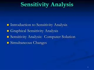
2. Outline • Definitions and requirements • Suggested practices http://www.jrc.cec.eu.int/uasa

3. Why uncertainty and sensitivity analyses? http://www.jrc.cec.eu.int/uasa

4. Why sensitivity analysis? Would you go to an orthopaedist who did not use X-rays? (J.M. Furbinger) http://www.jrc.cec.eu.int/uasa

5. Why sensitivity analysis? Sometime scientific theories compete as to which best describe the evidence. This competition takes place in the space of uncertainties (otherwise there would be no competition). Sensitivity analysis can help make the overall appreciation of the merits of each theory clearer, by mapping a theory’s assumptions onto its inferences.   This may even lead to the falsification of one of the theories.  http://www.jrc.cec.eu.int/uasa

6. Why sensitivity analysis? Sometime scientific information  feeds into the policy process. When this is the case, all parties manipulate uncertainty.  Uncertainty cannot be resolved into certitude in most instances. Instead, transparency can be offered by sensitivity analysis. Transparency is what is needed to ensure that the negotiating parties do retain science as an ingredient of decision making. http://www.jrc.cec.eu.int/uasa

7. A Definition [Global*] sensitivity analysis: “The study of how the uncertainty in the output of a model (numerical or otherwise) can be apportioned to different sources of uncertainty in the model input” *Global could be an unnecessary specification, were it not for the fact that most analysis met in the literature are local or one-factor-at-a-time … but not at this workshop! http://www.jrc.cec.eu.int/uasa

8. OAT methods One factor at a time methods are those whereby each input variable is varied or perturbed in turn and the effect on the output measured. http://www.jrc.cec.eu.int/uasa

9. OAT methods – derivatives Effect on Y of perturbing xj around its nominal value Relative effect on Y of perturbing xj by a fixed fraction of its nominal value Relative effect on Y of perturbing xj by a fixed fraction of its standard deviation http://www.jrc.cec.eu.int/uasa

10. OAT methods Derivatives can be computed efficiently using an array of different analytic, numeric or coding techniques (Turanyi and Rabitz 2000). When coding methods are used, computer programmes are modified (e.g. inserting lines of code and coupling with libraries) so that derivatives of large set of variables can be automatically computed at runtime (Grievank, 2000; Cacuci, 2005). http://www.jrc.cec.eu.int/uasa

11. OAT methods While derivatives are valuable for an array of estimation, calibration, inverse problem solving, and related settings, their use in sensitivity analysis proper is modest in the presence of finite factors uncertainty and non linear models. http://www.jrc.cec.eu.int/uasa

12. OAT methods A search was made on January 2004 on Science Online, a companion web side of Science magazine (impact factor above 20!). All articles having “sensitivity analysis” as a keyword (23 in number) were reviewed. All articles either presented what we would call an uncertainty analysis (assessing the uncertainty in Y) or performed an OAT type of sensitivity analysis. http://www.jrc.cec.eu.int/uasa

13. OAT methods • Among practitioners of sensitivity analysis this is a known problem – non OAT approaches are considered too complex to be implemented by the majority of investigators. • Among the global methods used by informed practitioners are: • variance based methods, already described, • the method of Morris, • various types of Monte Carlo filtering. http://www.jrc.cec.eu.int/uasa

14. Uncertainty analysis = Mapping assumptions onto inferences Sensitivity analysis = The reverse process Simplified diagram - fixed model

15. Sensitivity analysis can be used to gauge what difference a policy (or a treatment) makes given the uncertainties. An application to policy

16. Sources: A compilation of practices (2000), a ‘primer’ (2005). A third book, for students, is being written again for Wiley. SIMLAB can be freely downloaded from the web. http://www.jrc.cec.eu.int/uasa

17. The critique of models <-> Uncertainty <<I have proposed a form of organised sensitivity analysis that I call “global sensitivity analysis” in which a neighborhood of alternative assumptions is selected and the corresponding interval of inferences is identified. Conclusions are judged to be sturdy only if the neighborhood of assumptions is wide enough to be credible and the corresponding interval of inferences is narrow enough to be useful.>> Edward E. Leamer, 1990 See http://sensitivity-analysis.jrc.cec.eu.int/ for all references quoted in this talk. http://www.jrc.cec.eu.int/uasa

18. Our suggestions on useful requirements Requirement 1. Focus About the output Y of interest. The target of interest should not be the model output per se, but the question that the model has been called to answer. To make an example, if a model predicts contaminant distribution over space and time, it is the total area where a given threshold is exceeded at a given time which would play as output of interest, or the total health effects per time unit. http://www.jrc.cec.eu.int/uasa

19. Requirement 1 - Focus • … about the output Y of interest (continued) • One should seek from the analyses conclusions of relevance to the question put to the model, as opposed to relevant to the model, e.g. • Uncertainty in emission inventories [in transport] are driven by variability in driving habits more than from uncertainty in engine emission data. • In transport with chemical reaction problems, uncertainty in the chemistry dominates over uncertainty in the inventories. http://www.jrc.cec.eu.int/uasa

20. Requirement 1 - Focus • A few words about the output Y of interest (continued) • Engineered barrier count less than geologicalbarriers in radioactive waste migration. http://www.jrc.cec.eu.int/uasa

21. Requirement 1 - Focus On the output Y of interest (continued) An implication of what just said is that models must change as the question put to them changes. The optimality of a model must be weighted with respect to the task. According to Beck et al. 1997, a model is “relevant” when its input factors actually cause variation in the model response that is the object of the analysis. http://www.jrc.cec.eu.int/uasa

22. Requirement 1 - Focus Bruce Beck’s thought, continued Model “un-relevance” could flag a bad model, or a model unnecessarily complex, used to fend off criticism from stakeholders (e.g. in environmental assessment studies). As an alternative, empirical model adequacy should be sought, especially when the model must be audited. http://www.jrc.cec.eu.int/uasa

23. Requirements Requirement 2. Multidimensional averaging. In a sensitivity analysis all known sources of uncertainty should be explored simultaneously, to ensure that the space of the input uncertainties is thoroughly explored and that possible interactions are captured by the analysis. (as in EPA’s guidelines). http://www.jrc.cec.eu.int/uasa

24. Requirement 2 – Multidimensional Averaging Some of the uncertainties might be the result of a parametric estimation, but others may be linked to alternative formulations of the problems, or different framing assumptions which might reflect different views of reality, as well as different value judgements posed on it. http://www.jrc.cec.eu.int/uasa

25. Requirement 2 – Multidimensional Averaging Most models will be linear if one or few factors are changed in turn, and/or the range of variation is modest. Most models will be non linear and/or non additive otherwise. http://www.jrc.cec.eu.int/uasa

26. Requirement 2 – Multidimensional Averaging Typical non linear problems are multi-compartment or -phase, multi process models involving transfer of mass and/or energy, coupled with chemical reaction or transformation (e.g. filtration, decay…). Our second requirement can also be formulated as: sensitivity analysis should work regardless of the properties of the model. It should be “model free”. http://www.jrc.cec.eu.int/uasa

27. Requirement 2 – Multidimensional Averaging Averaging across models. When there are observations available to compute posterior probabilities on different plausible models, then sensitivity analysis should plug into a Bayesian model averaging. http://www.jrc.cec.eu.int/uasa

28. Requirements Requirement 3. Important how?. Another way for a sensitivity analysis to become irrelevant is to have different tests thrown at a problem, and different factors importance rankings produced without clue as to what to believe. To avoid this, a third requirement for sensitivity analysis is that the concept of importance be defined rigorously before the analysis. http://www.jrc.cec.eu.int/uasa

29. Requirements Requirement 4. Pareto. Most often input factors importance is distributed as wealth in nations, with few factors making all the uncertainty and most factors making a negligible contribution to it. A good method should do more than rank the factors, so that this Pareto effect, if present, can be revealed. Requirement 5. Groups. When factors can be logically grouped in subsets, it is handy if the sensitivity measure can be computed for the group, with the same meaning as for the individual factor (as done by all speakers at this workshop when discussing variance based methods). … http://www.jrc.cec.eu.int/uasa

30. Incentives for sensitivity analysis • Sensitivity analysis can • surprise the analyst, • find technical errors, • gauge model adequacy and relevance, • identify critical regions in the space of the inputs (including interactions), • establish priorities for research, • simplify models, • verify if policy options (or treatments) make a difference or can be distinguished. • anticipate (prepare against) falsifications of the analysis • … http://www.jrc.cec.eu.int/uasa

31. Incentives for sensitivity analysis • … there can be infinite applications as modelling setting are infinite. A model can be: • Prognostic or diagnostic • Exploratory or consolidative (see Steven C. Bankes – ranging from an accurate predictor to a wild speculation) • Data driven (P. Young) or first-principle, i.e. parsimonious (usually to describe the past) or over-parametrised (to allow features of the future to emerge) • Disciplinary (physics, genetics, chemistry…) or statistical • Concerned with risk, control, optimisation, management, discovery, benchmark, didactic, … http://www.jrc.cec.eu.int/uasa

32. Incentives for sensitivity analysis What methods would meet these promises and fulfil our requirements? The next section will try to introduce the methods, and some of their properties, using a very simple example. http://www.jrc.cec.eu.int/uasa

33. Practices • We try to build a case for the use of a set of methods which in our experience met the requirements illustrated thus far. These are • Variance Based Methods • Morris method • Monte Carlo filtering and related measures http://www.jrc.cec.eu.int/uasa

34. The first example introduces the variance based measures and the method of Morris. http://www.jrc.cec.eu.int/uasa

35. A self-evident problem, to understand the methods applied to it. A simple linear form: Y is the output of interest (a scalar), j are fixed coefficients Zj are uncertain input factors distributed as:

36. Given the model Y will also be normally distributed with parameters:

37. Additional assumptions for

38. According to most of the existing literature, SA is: which would give for our model of Y: =For Our Model FOM http://www.jrc.cec.eu.int/uasa

39. Hence the factors’ ordering by importance would be based on although … we don’t go far with

40. A better measure could be (IPCC suggestion): which, applied to our model, gives: FOM http://www.jrc.cec.eu.int/uasa

41. Comparing : with we get: … but only because our model is linear! The variance ofY decomposed!

42. We have to move into “exploration”, e.g. via Monte Carlo by generating a sample and estimating Y to get:

43. Regressing the y’ s on the zi’s we obtain a regression model where asymptotically Most regression packages will already provide the regression in terms of standardised regression coefficients FOM http://www.jrc.cec.eu.int/uasa

44. Comparing with we conclude that for linear models http://www.jrc.cec.eu.int/uasa

45. The variance ofY decomposed (again!) Summarising our results so far: for linear models … but something is in the bag also for non linear models. http://www.jrc.cec.eu.int/uasa

46. For non linear models but: 1) At least we know how much non linear the model is, and can decompose the fractionof the model variance that comes from linear effects: http://www.jrc.cec.eu.int/uasa

47. 2) The coefficients offer a measure of sensitivity that is multi-dimensionally averaged, unlike the .For linear model this does not matter but it does, and a lot for non linear ones. The drawback is when ; typically can be zero or near it for non monotonic models. http://www.jrc.cec.eu.int/uasa

48. Wrapping up the results so far obtained. We like the idea of decomposing the variance of the model output of interest according to source (the input factors), but would like to do this for all models, independently from their degree of linearity or monotonicity. We would like a model-free approach. http://www.jrc.cec.eu.int/uasa

49. How do we get there? … a different path is needed. If I could determine the value of an uncertain factor, e.g. one of our and thus fix it, how much would the variance of the output decrease? E.g. imagine the true value is and hence we fix it obtaining a “reduced” conditional variance: http://www.jrc.cec.eu.int/uasa

50. is a weak measure to rank the input factors, as (i) I do not know where to fix the factor, and (ii) for non-linear model one could have but this difficulty can be overcome by averaging this over the distribution of the uncertain factor http://www.jrc.cec.eu.int/uasa