Download
1 / 92
920 likes | 946 Views
Discover the basics of analog video, from continuous signals and electron beams to screen phosphors and persistence of vision. Explore frame rates, interlacing, display standards like NTSC, PAL, and SECAM, as well as video representation, digitization processes, and network protocols in the world of digital video. Learn about H.261 video compression standards and CIF formats, and dive into the concepts of interlacing, temporal rates, and quality in video production.

E N D
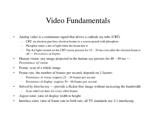
Video Fundamentals • Analog video is a continuous signal that drives a cathode ray tube (CRT) • CRT: an electron gun fires electron beams to a screen pasted with phosphors • Phosphor emits a dot of light when the beam hits it • The dot light created on the CRT screen persists for 15 – 20 ms even after the electron beam is off --- Persistence of display • Human vision: any image projected to the human eye persists for 40 – 50 ms --- Persistence of vision • Frame: scan of a whole image • Frame rate: the number of frames per second; depends on 2 factors: • Persistence of vision: requires 25 – 30 frames per second • Persistence of display: requires 50 – 60 frames per second • Solved by Interlacing --- provide a flicker-free image without increasing the bandwidth • Scan odd/even lines for every other frames • Aspect ratio: ratio of display width to height • Interlace ratio: ratio of frame rate to field rate; all TV standards use 2:1 interlacing
TV Standards • NTSC (National Television Standards Committee): US, Canada, Japan, Korea • SECAM (Systeme Electronique Color Avec Memoire): France and Eastern Europe • PAL (Phase Alternate Line): Rest of Europe, South America, Australia, rest of Asia Standard Vertical Res Frame Rate Horizon. Res. Interlace Aspect Bandwidth NTSC 525 30 340 2:1 4:3 4.2 MHz SECAM 625 25 409 2:1 4:3 6.0 MHz PAL 625 25 409 2:1 4:3 5.5 MHz(UK) 5.0 MHz (elsewhere)
Analog Video Representation • Video composed of luma and chroma signals • Composite video combines luma and chroma together • NTSC: composite = Y + I cos(F) + Q sin(F) or composite = Y + Ucos(F) + Vsic(F) • PAL: composite = Y + U sin(F) + V cos(F) • F: carrier frequency; NTSC: F = 3.58MHz; PAL: F = 4.43MHz; for analog video, YIQ is equivalent to YUV with a 33 degree rotation and an axis flip in the UV plane • Component video sends them separately • HVC, RGB, YUV, YIQ, Y C_R C_B (used for most compressed representations)… • Component video takes more bandwidth than composite video • Systems are represented by Vertical Resolution/Frame Rate (or Double)/Interlace Rate • NTSC: 525/60/2:1 • PAL: 625/50/2:1 • Video recording standards: • VHS • BETA • VIDEO-8
Digitizing Video • Digital video uses discrete numeric values, just like digital imagery • Signal is sampled • Samples are quantized • Frames are represented as pixel arrays • Line sampling • 4:2:2 is referred to as broadcast quality • 4:1:1 is referred to as VHS quality • 4:2:0 means 2:1 horizontal and 2:1 vertical downsampling. Y Y Y Y Y 4:4:4 CR/CB CR/CB CR/CB CR/CB CR/CB 1 Y = 1 Cb = 1 Cr Y Y Y Y Y 4:2:2 CR/CB CR/CB CR/CB 2:1 horizontal downsampling no vertical downsampling Y Y Y Y Y 4:1:1 CR/CB 4:1 horizontal downsampling no vertical downsampling
Digital Block Structure • 4:2:2 YCRCB • 16x16 macroblocks • 8x8 pixel blocks • 8 bits/sample = 16 bits/pixel = 4K bits/macroblock • 4:1:1 YCRCB • 3K bits/macroblock • 12 bits/pixel Y1 Y2 CB1 CR1 Y3 Y4 CR2 CB2 Y1 Y2 CR CB Y3 Y4
Digital Video Representations • Digital composite video • 14.3 MB/s data rate, either parallel or serial • Subsampled color signals 4:2:2 • Each pixel: Y0+I0, Y1+Q1, Y2+I2, Y3+Q3, … • Digital component video • Maintain separate signals for luminance and color • 27 MB/s data rate, either parallel or serial • Subsampled color signals 4:2:2 • Each pixel is 2 bytes: (CB0, Y0), (CR1, Y1), (CB2, Y2), (CR3, Y3), … • Network protocols and their bit-rate regimes Conventional telephone 0.3 – 56 Kb/s Fundamental bandwidth unit of telephone company (DS-0) 56 Kb/s Integrated-services digital network (ISDN) 64 – 144 Kb/s Personal computer local-area network 30 Kb/s T-1 (multiple of DS-0 = DS-1) 1.5 Mb/s T-2 (multiple of DS-0 = DS-2) 6.3 Mb/s Ethernet (packet-based local-area network) 10 Mb/s T-3 (multiple of DS-0 = DS-3) 45 Mb/s Fiber-optic ring-based network 100 – 200 Mb/s
H.261 Standard • CCITT recommended video compression standard for videoconferencing and videophone services over ISDN (Integrated Services Digital Network) in 1990 • Data rate at p x 64 Kbps, p = 1, … , 30 • P=1 for low quality videophone services (e.g., 48 Kbps for video and 16 Kbps for audio) • p6 for videoconferencing services • P=30 (1.92Mbps) is the maximum bit rate VHS-quality or higher images • In addition to the compression standard, H.261 also offers 2 important features: • Specifies a maximum coding delay of 150 ms (delays > 150 ms do not give viewers the impression of direct visual feedback) • Amenable to low-cost VLSI implementation • Designed compatible with both 625 lines and 525 lines TV standards • Common Intermediate Format (CIF) • Quarter of CIF (QCIF) • Input Image Formats: CIF QCIF # active pixels/line [Lum(Y), Chroma(U, V)] [360, 180] [180, 90] # active lines/image [Lum(Y), Chroma(U, V)] [288, 144] [144, 72] Interlacing 1:1 1:1 Temporal rate 30,15,10 or 7.5 30,15,10, or 7.5 Aspect ratio 4:3 4:3
Data Structures of H.261 • Hierarchical structure: • Video consists of picture layer --- each picture is a frame • Picture consists of group of blocks (GOB) layer --- fixed number of blocks • GOB consists of macroblocks (MB) layer --- fixed number of blocks • MB consists of block layer --- fixed number of blocks • Each layer has a header consisting of a set of parameters describing the layer • MB is the smallest unit of data for selecting a compression mode • Every 4 Luma blocks are coupled with 1 block of chroma (U and V) • Subsampled one chroma value for every two Luma value in both dimensions • MB header contains the MB address, the compression mode of this MB, and the data • GOB layer always consists of 33 macroblocks arranged as a 3x11 matrix • Picture layer consists of the header followed by the data of GOBs • Composition of the picture layer: Format # GOB/frame # MB/GOB Total # MB/frame CIF 12 33 396 QCIF 3 33 99
Video Compression of H.261 • H.261 has two compression modes • Intra mode --- similar to JPEG still-image compression --- based on block-by-block DCT • Inter mode --- a temporal prediction is employed with or without motion compensation (MC) followed by DCT coding of the interframe prediction error • Each mode offers several options (changing the quantization scale parameter, using MC) • Compression algorithm: • Estimate a motion vector (MV) for each MB • No specific motion estimation method is defined, and MC is optional • Usually 16x16 luminance block based matching • Decoder accepts one integer-valued MV per MB whose components do not exceed 15 • Select a compression mode for each MB based on a criterion defined by displaced block difference (dbd): dbd(x, k) = b(x, k) – b(x-d, k-1) where b(.,.) denotes a block, x and k are pixel coordinates and time index, respectively, and d is the MC defined for the kth frame relative to the (k-1)st frame; if d = 0, dbd becomes macroblock difference (bd) • Process each MB to generate a header followed by a data bitstream that is consistent with the compression model chosen
Compression Mode of H.261 • Selection depends on answers to several key questions: • Should a MC be transmitted? • Inter vs. Intra compression? • Should the quantizer step size be changed? • Specifically, selection is based on the following values • Variance of the original macroblock • The macroblock difference (bd) • The displaced macroblock difference (dbd) • Selection algorithm: • If the variance of dbd < bd as determined by a threshold, select mode Inter + MC, and the MV needs to be transmitted as side information • Else, MV will not be transmitted; if the original MB has a smaller variance, select Intra mode where DCT of each 8x8 block of the original picture elements are computed; else, select Inter mode (with zero MV), and the difference blocks (prediction error) are DCT encoded
H.261 Coding Scheme • In each MB, each block is 64 point DCT coded; this applies to the four luminance blocks and the two chroma blocks (U and V) • A variable thresholding is applied before quantization to increase the number of zero coefficients; the accuracy of the coefficients is 12 bits with dynamic range in [-2048, 2047] • Within a MB the same quantizer is used for all coefficients except for the Intra DC; the same quantizer is used for both luminance and chromainance coding; the Intra DC coefficient is separately quantized • After quantization, coefficients are zigzag coded by a series of pairs (the run length of the number of zeros preceding the coefficient, the coefficient value) • Example: 3 0 0 0 0 0 0 0 2 0 0 0 0 0 0 0 0 0 0 0 0 0 0 0 0 0 0 0 0 0 0 0 1 0 0 0 0 0 0 0 … (0, 3), (1, 2), (7, 1), EOB • In most implementations the quantizer step size is adjusted based on a measure of buffer fullness to obtain the desired bit rate; the buffer size is chosen not to exceed the maximum allowable coding delay (150 ms)
MPEG Standard • Only specified as a standard --- actual CODECs are up to many different algorithms, most of them are proprietary • All MPEG algorithms are intended for both applications • Asymmetric: frequent use of decompression process while compression process is performed once (e.g., movie on demand, electronic publishing, e-education, distance learning) • Symmetric: equal use of compression and decompression processes (e.g., multimedia mail, video conferencing) • Decoding is easy • MPEG1 decoding in software on most platforms • Hardware decoders widely available with low prices • Windows graphics accelerators with MPEG decoding now entering market (e.g., Diamond) • Encoding is expensive • Sequential software encoders are 20:1 real-time • Real-time encoders use parallel processing • Real-time hardware encoders are expensive • MPEG standard consists of 3 parts: • Synchronization and multiplexing of video and audio • Video • Audio
MPEG-1 Standard • Unlike JPEG, does not define specific algorithms needed to produce a valid data stream • Similar to H.261, does not standardize a motion estimation algorithm or a criterion for selecting the compression mode • Offers the following application-specific features: • Random access is essential in any video storage application • Fast forward/backward search refers to scanning the compressed bit stream and to display only selected frames to obtain fast forward or backward search; backward playback might also be necessary • Reasonable delay of about 1 second to give the impression of interactivity in unidirectional video access (as opposed to strict 150 ms delay imposed in H.261 to maintain bidirectional interactivity) • Considers progressive (noninterlaced) video only MPEG Standard Input Format (SIF) is defined: • (Y, Cr, Cb) color space • Y: 352 pixels x 240 lines x 30 frames; chroma components subsampled by 2 in both dimensions • 8 bits/pixel for both luminance and chrominance • Set of hard constraints for maximum hardware implementation • Max. #pixels/line: 720; Max. #lines/frame: 576; Max. #frames/second: 30 • Max. #MBs/frame: 396; Max. #MBs/second: 9900; Max. bitrate: 1.86Mbps; • Max. decoder buffer size: 376,832 bits
MPEG-1 Data Structure • Similar to H.261, follows a hierarchical structure with six layers • Sequence layer --- video data consists of sequences, each of which is several groups of pictures • Group of pictures layer --- GOP consists of pictures or frames • Pictures layer --- consists of slices • Slice layer --- consists of MBs • MB layer --- consists of blocks • Block layer --- the smallest unit of DCT coding • Headers are defined for the layers of sequence, GOP, picture, slice, and MB • What layer it is • The number of units next layer has • The actual data stream of the next layer
Frame Structures • I frames (intra images): • Self-contained and coded using a DCT-based technique similar to JPEG • Used as random-access points in MPEG-1 streams • Low compression ratio within MPEG-1 • P frames (predicted images): • Coded using forward predictive coding where the actual frame is coded with reference to a previous frame (I or P) • Compression ratio is significantly higher than I • B frames (bidirectional or interpolated images): • Coded using two reference frames, a past and a future frames (which may be I or P) • Highest compression ratio • The decoding order may differ from the encoding order: • Example: I B B B P B B B I • If the MPEG sequence is transmitted over the network, the actual decoding order is: 1, 5, 2, 3, 4, 9, 6, 7, 8 • Empirically, best sequence turns out to be • I B B P B B P B B I
Motion Vector Estimation • Block-wise motion vectors are estimated (rather than pixel-wise, which is the difference between optical flow estimation in image understanding and motion vector estimation in MPEG) • The estimation of each block’s motion, however, is done through pixel-wise, or simplified pixel-wise correlation • In interframe compression modes, a temporal prediction is formed, and the prediction error is DCT encoded; two types of temporal prediction modes allowed in MPEG-1: • P-pictures: forward prediction with respect to a previous I or P frame • B-pictures: bidirectional prediction with respect to previous and following I or P frames • Just forward prediction • Just backward prediction • Both forward and backward predictions • Trade-offs associated with B-pictures: • Two frame store buffers are needed at the encoder and decoder, since at least two reference frames need to be decoded first • If too many B-pictures are used, • The distance between the two reference frames increases, resulting in less temporal correlation between them, and hence more bits are required to encode the reference frames • Longer coding delay
Comparison b/w H.261 and MPEG-1 H.261 MPEG-1 Sequential access Random access One basic frame rate Flexible frame rate CIF and QCIF images only Flexible image size I and P frames only I, P, and B frames MC over 1 frame MC over 1 or more frames 1 pixel MV accuracy ½ pixel MV accuracy Variable threshold + uniform quantization Quantization matrix (predefined) No GOP structure GOP structure GOB structure Slice structure
Differences b/w MPEG-2 Video and MPEG-1 Video • Bandwidth requirement: MPEG-1 --- 1.2 Mbps MPEG-2 2-20 Mbps • MB structures: alternative subsampling of the chroma channels 3 subsampling formats • MPEG-2 accepts both progressive and interlaced inputs • Progressive video: like MPEG-1, all pictures are frame pictures • Interlaced video: encoder consists of a sequence of fields; two options: • Every field is encoded independently (field pictures) • Two fields are encoded together as a composite frame (frame pictures) • Allowed to switch between frame pictures and field pictures on a frame to frame basis frame encoding is preferred for relatively still images while field encoding is preferred for images with significant motion 4:4:4 4:2:2 4:2:0 1 MB = 6 blocks (4Y,1Cr,1Cb) 1 MB = 8 blocks (4Y,2Cr,2Cb) 1 MB = 12 blocks (4Y,4Cr,4Cb)
MPEG-4 • Finalized in October of 1998; available in standards in early 1999 • Technical features: • Represent units of aural, visual, or audiovisual content, called “media objects”. These media objects can be of natural or synthetic origin; this means they could be recorded with a camera or microphone, or generated with a computer • Describe the composition of these objects to create compound media objects that form audiovisual scenes • Multiplex and synchronize the data associated with media objects, so that they can be transported over network channels providing a QoS appropriate for the nature of the specific media objects • Interact with the audiovisual scene generated at the receiver’s end • Enables • Authors to produce content with greater reusability and flexibility • Network service providers to have transparent information to maintain QoS • End users to interact with content at higher levels within the limits set by the authors
MPEG History • MPEG-1 is targeted for video CD-ROM • MPEG-2 is targeted for Digital Television • MPEG-3 was initiated for HDTV, but later was found to be absorbed into MPEG-2 abandoned • MPEG-4 is targeted to provide the standardized technological elements enabling the integration of the production, distribution, and content access paradigms of the fields of digital television, interactive graphics, and interactive multimedia • MPEG-7, formally named “Multimedia Content Description Interface”, is targeted to create a standard for describing the multimedia content data that will support some degree of interpretation of the information’s meaning, which can be passed onto, or accessed by, a device or a computer code; MPEG-7 is not aimed at any one application in particular; rather, the elements that MPEG-7 standardizes will support as broad a range of applications as possible • MPEG-21 is now under design and review
Design of Stream Video Server & Client • Whole system has two parts: server and clients • Clients may be multiple clients • Broadcast model • Server responsible for listening to the request from clients, and launches threads to serve clients • Client sends request to server • If request approved, client starts threads to receive data, and sends a start message to server to start displaying video session • Upon receiving the start message from the client, server begins to read data from disk files and sends them to the client through network
Server AdmittedClientSet AdmittedClient Network Video Sending Thread Feedback Thread Disk Read Thread
Server, Cont’d • A dialog based MFC application, written in Visual C++ 6.0 under Windows 2000 • CStreamVideoServerApp is the class of application, which has a data member named StreamVideoClientSet, a pointer to the AdmittedClientSet class • AdmittedClientSet keeps track of all the admitted clients • Each AdmittedClient has a video buffer with two threads • Video sending thread --- sending out video • Feedback thread --- gets feedback messages from client • DiskReadThread serves all clients • Always browses over AdmittedClientSet • Read data from disk files • Write data to buffers of each AdmittedClient • If a buffer is full, DiskReadThread does not wait, and skip the buffer moving to the next one • Feedback messages are used to synchronize the transmission between server and client • At the beginning, CListenAdSocket is started to listen to requests; when a request is received, creates a CServerAdSocket to serve the client; CServerAdSocket reads the request from the client and processes it; if the request is approved, it adds a new AdmittedClient to the AdmittedClientSet and starts two threads in the AdmittedClient; meanwhile, DiskReadThread is started to serve all the AdmittedClient.
Client MultiMediaRealTimeStream Video Receiving Thread Video Assemble Thread File Buffer Feedback Thread
Client, Cont’d • Each client has MultiMediaRealTimeStream object, responsible for getting video from server and sending feedback messages back to server, as well as assembling the file (for simulation of playing the video) • When opened, asks for admission; if approved, start three threads: • Video receiving Thread (receive video/audio from packets) • Video assemble Thread (assemble data into a file) • Feedback Thread (synchronize server sending and client receiving data)
Buffer Management Writable items Read pointer Write pointer Readable items
Synchronization b/w Server & Client • Server starts to send data every Interval time • Client receives data and puts them into the client buffer • The client buffer has a threshold H • If the data in the buffer is less than H percent, the client sends a FASTER message to server • After server gets FASTER, decreases Interval • Client keeps sending FASTER to server till the client buffer reaches H • Client sends SLOWER message to server • Server increases Interval after receiving SLOWER • Finally the client buffer is kept around H
Multimedia Databases • What is an Multimedia Database Management System? • A framework that manages different types of data potentially represented in a wide diversity of formats on a wide array of media sources; must have the ability to • Uniformly query data represented in different formats • Simultaneously conduct classical database operations across different data formats stored in the database • Retrieve media objects from a local storage device in a smooth, jitter-free manner • Take an answer to a query and present the answer to users in terms of audio-visual media • Deliver this representation such that quality of service requirements are satisfied • Key differences between Multimedia databases and traditional databases • Data types • Structured data vs. non-structured data • Indexing --- Matching --- Retrieval cycle • Exact vs. inexact matching --- similarity • Storage issues • Presentation and delivery issues • Different data structures • K-d trees • Point Quadtrees • MX Quadtrees • R-trees • TV trees
K-d trees • Store k dimensional point data • Not used to store region data even though range information may be inferred from • Node structure for a 2-d tree: nodetype = record INFO: infotype; XVAL: real; YVAL: real; LLINK: ^nodetype; RLINK: ^nodetype end • INFO field is a user-defined type of information • XVAL and YVAL denote the coordinates of a point associated with the node in 2-d trees • LLINK and RLINK fields point to two children of this node • Each point in the tree represents a hyperplane perpendicular to the ith dimension of the k-d space at the ith coordinate of this point; this hyperplane separates the region implicitly represented by this point
Definition of 2-d Trees • The level of nodes is defined numerically starting 0 at the root • A 2-d tree is any binary tree satisfying the following conditions: • If N is a node in the tree such that level(N) is even, then every node M in the subtree rooted at N.LLINK has the property that M.XVAL < N.XVAL; every node P in the subtree rooted at N.RLINK has the property that P.XVAL N.XVAL • If N is a node in the tree such that level(N) is odd, then every node M in the subtree rooted at N.LLINK has the property that M.YVAL < N.YVAL; every node P in the subtree rooted at N.RLINK has the property that P.YVAL N.YVAL • Example • Given points in the order: A B C D E (19, 45) (40, 50) (38, 38) (54, 35) (4, 4) • 2-d tree: 19, 45 4, 4 40, 50 38, 38 54, 35
Insertion and Search in 2-d Trees • To insert a node N into a tree pointed to by T • Check to see if N and T agree on their XVAL and YVAL fields • If so, just overwrite node T and stop • Else, branch left if N.XVAL < T.XVAL and branch right otherwise (note that this time the level is 0) • Suppose P denotes the child we are examining. If N and P agree on their XVAL and YVAL fields, then overwrite node P and stop; else branch left if N.YVAL < P.YVAL and branch right otherwise (note that this time the level is 1) • Repeat this procedure till stop, branching on XVAL when we are at even levels in the tree, or on YVAL when we are at odd levels in the tree • Example: add the sixth node F: (15, 9) to the previous 2-d tree 19, 45 4, 4 40, 50 15, 9 38, 38 54, 35
Deletion in 2-d Trees • Suppose T is a 2-d tree, and (x, y) refers to a point that we wish to delete from the tree • Search for the node N in T that has N.XVAL = x and N.YVAL = y • If N is a leaf node, then set the appropriate field (LLINK or RLINK) of N’s parent to NIL and return N to available storage; stop • Else, either the subtree rooted at N.LLINK (called Tl) or the subtree rooted at N.RLINK (called Tr) is non-empty • Find a “candidate replacement” node R that occurs in either Tl or Tr • Replace all of N’s non-link fields with those of R • Recursively delete R from Tl or Tr (Note that this recursion is guaranteed to terminate as either Tl or Tr has strictly smaller height than the original tree T) • Finding candidate replacement • The desired replacement node R must bear the same spatial relationship to all nodes P in both Tl and Tr that N bore to P; i.e., if P is to the SW of N, P must be to the SW of R, etc. This means that R must satisfy: • Every node M in Tl is such that M.XVAL < R.XVAL if level(N) is even and M.YVAL < R.YVAL if level(N) is odd • Every node M in Tr is such that M.XVAL R.XVAL if level(N) is even and M.YVAL R.YVAL if level(N) is odd
Candidate Replacement Algorithm • If Tr is not empty, and level(N) is even, then any node in Tr that has the smallest possible XVAL field in Tr is a candidate replacement node (what if there are several candidates with the same smallest XVAL?); similarly, if Tr not empty, and level(N) is odd, node in Tr with smallest YVAL; then recursively delete R resulting Tr Tr’ • If Tr is empty, then we might not be able to find a candidate replacement node from Tl (Why?); In this case, find the node R’ in Tl with the smallest possible XVAL field and replace N with R’ (why?), if level(N) is even; similarly, find R’ in Tl with the smallest YVAL and replace N with R’, if level(N) is odd • Then set N.RLINK = N.LLINK and set N.LLINK = nil; recursively delete R’
Range Queries in 2-d Trees • A range query w.r.t. a 2-d tree T is a query that specifies a point (xc, yc), and a distance r • The answer to such a query is the set of all points (x, y) in the tree T such that (x, y) lies within the distance r of (xc, yc) • Recall that each node N in a 2-d tree implicitly represents a region R_N; if the circle specified in a range query has no intersection with R_N, then there is no point to search the subtree rooted at node N • Range query algorithm: • Need to modify the nodetype data structure to include range boundary information for each area a point implicitly represents • RangeCheck(T, R) where T: 2-d tree; R: (xc, yc, r) range if T R, stop and output if T R, stop and output T else RangeCheck(Tl, R); RangeCheck(Tr, R); • Note that the range information is used to expedite the search by exclusion; but for the final checking whether a point is inside the range, the coordinate information needs to be used
Search By Exclusion • Important search technique --- especially for search in multimedia data structures • Tries to exclude impossible solutions as many as possible in each search step • Usually involves recursion Cut whole subtree
Point Quadtrees • Always split regions into four parts • In a 2-d tree, node N splits a region by drawing one line through the point (N.XVAL, N.YVAL); in a point quadtree, node N splits the region by drawing both a horizontal and a vertical line through the point (N.XVAL, N.YVAL) dividing the region into four quadrants: NW, SW, NE, SE, with each corresponding to a child of node N; quadtree nodes may have up to four children each • Node structure in a point quadtree: qdnodetype = record INFO: infotype; XVAL: real; YVAL: real; NW,SW,NE,SE: ^qdnodetype end
Operations in Point Quadtrees • Expand the node structure qdnodetype to a new node structure newqdnodetype qdnodetype = record INFO: infotype; XVAL: real; YVAL: real; XLB,XUB,YLB,YUB: real {-, + } NW,SW,NE,SE: ^qdnodetype end • When inserting a node N into the tree T, we need to ensure that: • If N is the root of T, then N.XLB = - , N.XUB = + , N.YLB = - , N.YUB = + • If P is the parent of N, then the following table describes what N’s XLB, YLB, XUB, YUB fields should be, depending on whether N is the NW, SW, NE, SE child of P Case N.XLB N.XUB N.YLB N.YUB N = P.NW P.XLB P.XVAL P.YVAL P.YUB N = P.SW P.XLB P.XVAL P.YLB P.YVAL N = P.NE P.XVAL P.XUB P.YVAL P.YUB N = P.SE P.XVAL P.XUB P.YLB P.YVAL
Operations in Point Quadtrees, Cont’d • When deleting an interior node N, we must find a replacement node R in one of the four possible subtrees of N, such that • Every other node R1 in N.NW is to the northwest of R • Every other node R2 in N.SW is to the southwest of R • Every other node R3 in N.NE is to the northeast of R • Every other node R4 in N.SE is to the southeast of R • In general, it may not always be possible to find such a replacement node; the worst case is that all the nodes in the tree need to be reinserted • Example: Quadtree of A, B, C, D, E. If delete A, C is the replacement; if add F:(50, 40), no replacement is possible for A A: (19, 45) SW NW SE NE E: (4, 4) C: (38, 38) B: (40, 50) SW NW SE NE SW NW SE NE SW NW SE NE D: (54, 35) F: (50, 40) SW NW SE NE SW NW SE NE
Range Search in Point Quadtrees • Similar to 2-d trees, a range query is represented by a center (xc, yc) and a radius distance r • Use the expanded point quadtree data structure which includes the boundary information for each region a point represents • So each node in a point quadtree represents a region • Do not search regions that do not intersect the circle defined by the query • A recursive algorithm similar to that in 2-d trees is able to take care of this search
MX-Quadtrees • For both 2-d trees and point quadtrees, the “shape” of a tree depends upon the order in which objects are inserted into the tree • The split regions are not even, depending upon where the point (N.XVAL, N.YVAL) is located inside the region represented by N • In MX-Quadtrees, the shape of a tree is independent of the number of nodes present in a tree, as well as the order of insertion of these nodes • MX-Quadtrees also attempt to provide efficient deletion and search algorithms • Assume that an image is split up into a grid of size 2^k 2^k for some k --- a constant reflecting the desired granularity • Node Structure: exactly the same as that of point quadtrees, except that the root of an MX-Quadtree represents the region specified by XLB = 0, XUB = 2^k, YLB = 0, YUB = 2^k • When a region gets “split”, it gets split down the middle. Thus, if N is a node, and if w = N.XUB – N.XLB = N.YUB – N.YLB, the region of the four possible children of N are Child XLB XUB YLB YUB NW N.XLB N.XLB+0.5w N.YLB+0.5w N.YUB SW N.XLB N.XLB+0.5w N.YLB N.YLB+0.5w NE N.XLB+0.5w N.XUB N.YLB+0.5w N.YUB SE N.XLB+0.5w N.XUB N.YLB N.YLB+0.5w
Operations in MX-Quadtrees • All the points in a MX-Quadtree are located at the leaf level (i.e., level k); each point (x, y) in an MX-Quadtree represents a 1 1 region whose lower-left corner is (x, y) • The insertion/search operation is straightforward points will always be inserted at level k in the tree • The deletion operation is also fairly simple as all the points are at the leaf level • If a node becomes Nil for all the four children due to deletion of its children, collapse the node and set the child of the parent’s node as Nil • Repeat this process till reaching the root; the total time for deletion is O(k) • Maximum number of points in an MX-Quadtree is 2^(k+1) • Range queries in MX-Quadtrees: exactly the same as for point quadtrees except for the following two differences: • The constant of the XLB, XUB, YLB, YUB fields is different from that in the case of point quadtrees • Checking to see if a point is in the circle defined by a range query only needs to be preformed at the leaf level
PR-Quadtrees • In MX-Quadtrees, all leaves are at the same height --- balanced trees search, insertion, deletion time O(k) • Change the rule: • A region is split iff it has > 1 points • If only one point in a region, store the value in this node (i.e., this node is a leaf node) becomes unbalanced trees • Save search/insertion/deletion time
B Trees • A tree with order k, and a key ordering property satisfying the following restrictions: • Every node has at most k children • Every node, except for the root, has at least k/2 children • The root has at least 2 children, unless it is a leaf • All leaves are at the same level • A non-leaf node with m children contains m-1 keys; for each key, all keys in the left subtree < it, and all keys in the right subtree > it • Example: a B tree with order = 3 4 12 X X 3 X X 5 X 8 X X 15 X 18 X
R Trees • Proposed by Antonin Guttman in 1984 • Store rectangular regions of an image using minimum bounding box --- MBB • Good for spatial data access • Particularly useful in storing very large amounts of data on disk; provides a convenient way of minimizing the number of disk accesses • MBB disk page • Definition • Each R-tree has an associated order K • Each non-leaf R-tree node contains a set of at most K children and at least K/2 children, except for the root, i.e., the tree must be at least half full • If a node is a leaf, it is a rectangle; otherwise, it is a “group” of rectangles • Extension of B-trees
Operations of R Trees • Insertion is based on the least group area criterion; need to pay attention to “overflow” of a node • Deletion needs to pay attention to “underflow” of a node; this requires readjustment of the tree nodes multiple solutions may be available • MBBs are allowed to overlap • The node structure: rtnodetype = record Rec1, … , RecK: rectangle; P1, … , PK: ^rtnodetype end • Here “rectangle” also includes group of rectangles
Examples of R-Trees R6 R1 R7 R5 R4 R3 R8 R2 R9
R6 R1 R7 R5 R4 R3 R8 R2 R9 One Solution K = 4 R1 R2 R3 R4 R5 R6 R7 R8 R9
R6 R1 R7 R5 R4 R3 R8 R2 R9 Another Solution K = 4 R1 R2 R3 R4 R5 R6 R7 R8 R9 R3
What if delete R9? --- Solution 1 R6 R1 R7 R5 R4 R3 R8 R2 K = 4 R1 R2 R3 R4 R7 R6 R8 R5
What if delete R9? --- Solution 2 R6 R1 R7 R5 R4 R3 R8 R2 K = 4 R1 R2 R3 R4 R5 R6 R7 R8 R4