Download
1 / 16
160 likes | 432 Views
Numerical Modeling of Flow and Transport Processes Solving Incompressible isothermal flow in a lid-driven cavity using Comsol Software Joseph Addy 31103196 Supervised by Professor Manfred Koch. Motivation Introduction to COMSOL

E N D
Numerical Modeling of Flow and Transport Processes Solving Incompressible isothermal flow in a lid-driven cavity using Comsol Software Joseph Addy 31103196 Supervised by Professor Manfred Koch
Motivation • Introduction to COMSOL • Governing Equations for incompressible isothermal flow in a lid-driven cavity • Boundary and Initial conditions for Problem description • Mesh generation, contour velocity and Matlab results • Conclusion Table of Contents
Simulation is fast and delivers local and global information in details, for example the velocity field or pressure distribution in a pipe. • Simulation provides approximate solution to real problems and also cheaper. • Numerical modeling provides general knowledge and understanding for the mode of operation of products and processes Motivation
COMSOL Software • COMSOL Multiphysics software is a powerful finite element (FEM), partial differential equation (PDE) solution engine. The software has eight add-on modules that expand the capabilities in the following application areas: • AC/DC Module • Acoustics Module • Chemical Engineering • Earth Science • Heat transfer • MEMS (microelectromechanical systems) • RF • Structural Mechanics • The Multiphysics has CAD Import Module and the Material Library as supporting software
COMSOL Software Multiphysics implies multiple branches of physics can be applied within each model. Comsol facilitates all steps in the modeling begining with your geometry, meshing , specifying your physics ( subdomain and boundary conditions), solving and then visualizing your results. Comsol can solve problems in 1D, 2D, 3D and axial symmetries in 1 and 2D
From the application modes one chooses the type of problem to be solved and from the space dimension, the type of dimension. Comsol software
u=1, v=0 Problem description with boundary and initial conditions The square geometry is fixed at all three sides with walls ,except the top side where it is assumed to be moving with a specified velocity in the x direction. The pressure gradient is neglected in the problem u=v=0 u=v=0 u=v=0
Governing Equations for 2D incompressible Navier Stokes equation without volumetric forces
Mesh generation for steady state Mesh consists of 590 elements Refine mesh consists of 2360 elements
A Matlab program shows similar result as the comsol result for unsteady incompressible isothermal flow in a lid driven cavity Matlab program for unstedy Incompressible isothermal flow in a lid-driven cavity
For steady state problems with low Reynold`s numbers the fluid flows in the direction of pressure difference as been expected with vorticities at the lower corners of the square geometry. When the physical quantities such as the density and viscosity are too high the simulation system does not find consistency , which implies that the computation does not converge. • For the unsteady state simulation , an initial boundary condition must be given and also higher than zero, otherwise the result from comsol simulation are not reasonable. Conclusion
Heat transfer in condensation and Boiling : Karl Stephan • Convective Boiling and Condensation: Collier and Thome • Heat transfer: Gregory Nellis and Sanford Klein • Matlab for poisson equation: Professor Koch • Multiphysics modeling Comsol: Roger W. Pryor • Stanford University Lecture: Prof.Barba Lorenza • MIT matlab code for incompressible navier stokes equation: Prof. Gilbert Strang References