Download
1 / 16
160 likes | 304 Views
Spatial Reduction Algorithm for Numerical Modeling of Atmospheric Pollutant Transport. Yevgenii Rastigejev, Philippe LeSager. Michael P. Brenner, Daniel J. Jacob. Harvard University. April, 2007. Fast Region. Slow Region. Motivation.

E N D
Spatial Reduction AlgorithmforNumerical Modeling of Atmospheric Pollutant Transport Yevgenii Rastigejev, Philippe LeSager Michael P. Brenner, Daniel J. Jacob Harvard University April, 2007
Fast Region Slow Region Motivation Problem: There is an urgent need to improve significantly computational performance of the existing GEOS-Chem code motivated by difficulties with numerical simulation of immerging applications Solution: To create a multi-scale numerical algorithm which provides a significant (order of magnitude) reduction in computational cost Our algorithm is inspired by the observation that atmospheric emissions have most of their fast reactants and their quickly decomposing reaction products localized near the emitter, typically on the ground. Far from the emitter, the fast reactants do not play a significant role.
Slow or r Fast D Chemical source Solution: Spatial Reduction In the Slow region Fast Region– the species is fully accounted as a dependent variable in the system of transport equations Slow Region–the species concentration is found through extrapolation For the algorithm to be efficient: size Slow Region >> size Fast Region comp. cost Slow Region << comp. cost Fast Region
Gradual Spatial Reduction A B Domain partitioning for A and B Slow Slow Fast Fast 2 eqn 1 eqn A,B A 1 eqn B Consider a two species reaction system, comprised of chemicals A and B The central idea of our algorithm is to track a series of chemical boundary layers (CBL) within which the gradual,continuous spatial reduction is employed from the domain where the full mechanism is needed to the domain where the most simplified mechanism is sufficient.
Prerequisites for Spatial Reduction Numerical Method Fast Fast Slow Slow Fast if Slow otherwise Domain partitioning • Fast-Slow domain partitioning algorithm • Algorithms for Reduced Model construction • Matching procedure • Efficient methodology for adaptation in time
distance Slow exp. decay rate Fast exp. decaying concentration Reduced model – exponential extrapolation into Slow region Matching conditions matching procedure for concentration values and mass fluxes ensures good mass conservation and continuity properties of the numerical scheme
O3 O3 O3 NO2 NO2 NO2 NO NO NO OH OH OH HO2 HO2 HO2 chemical flux Chemical model oxidation of a number of C3H6 in an OH oxidizing atmosphere, with NOx serving as catalyst through the cycling of HOx radicals 15 chemical species and 24 reactions
Comparison of species distribution obtained by the spatial reduction algorithm (spheres and cubes) and conventional method (solid line) depicted in blue and red colors at and at correspondingly at time Max err = 2-3 % Average err = 0.5 % Slow Fast Fast – Slow domain partitioning for the atmosphere with horizontal shear layer flow at time
Some preliminary conclusions • A gradualcontinuous spatial reduction computational method for Atmospheric chemistry has been developed. • Unlike conventional time-scale separation methods, the spatial reduction algorithm allows to speed up not only a "chemical solver" but also advection-diffusion numerical integration. • The method produced accurate results at 5-6 times lower computational cost for the 2-dimensional Atmospheric chemistry problems tested. • Currently we are working on the algorithm implementation into GEOS-Chem three-dimensional solver. To be continued with three-dimensional description …
G-C Implementation Old SOLVER (SMVGEAR) New SOLVER (DLSODES)
Criteria for CBLs [ n ] > Threshold Values OR Net Production > 10-3 Max Value 54% of ODE solved averaged RMS error of 7.2% Run Time = 0.66 Full Resolution Case
Short lived species : Max error in the outskirts of concentration peaks
Transported tracer: Max error further away from concentration peaks.
To be continued… • BetterCBLs (combining absolute/relative criteria,discriminating b/w species, fine tuning) • Extrapolation mechanism will • substantially reduce the error in the slow region • noticeably reduce the size of the fast region • Full advantage of sparse structure • substantial speed up