An Introduction to Point Processes
390 likes | 595 Views
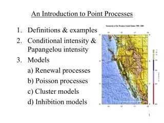
Definitions & examples Conditional intensity & Papangelou intensity Models a) Renewal processes b) Poisson processes c) Cluster models d) Inhibition models. An Introduction to Point Processes. Point pattern : a collection of points in some space.

An Introduction to Point Processes
E N D
Presentation Transcript
Definitions & examples • Conditional intensity & Papangelou intensity • Models • a) Renewal processes • b) Poisson processes • c) Cluster models • d) Inhibition models An Introduction to Point Processes
Point pattern: a collection of points in some space. Point process: a random point pattern. Centroids of Los Angeles County wildfires, 1960-2000
Marked point process: a random variable (mark) with each point. Hollister, CA earthquakes: locations, times, & magnitudes
Time series: Palermo football rank vs. time Marked point process: Hollister earthquake times & magnitudes
Antiquated definition: a point process N(t) is a right-continuous, Z+-valued stochastic process: --x-------x--------------x-----------------------x---x-x--------------- 0 t T N(t) = Number of points with times < t. Problem: does not extend readily to higher dimensions. Modern definition: A point process N is a Z+-valued random measure N(a,b) = Number of points with times between a & b. N(A) = Number of points in the set A.
More Definitions: • s-finite: finite number of pts in any bounded set. • Simple: N({x}) = 0 or 1 for all x, almost surely. (No overlapping pts.) • Orderly: N(t, t+ D)/D ---->p 0, for each t. • Stationary: The joint distribution of {N(A1+u), …, N(Ak+u)} does not • depend on u. • Notation & Calculus: • ∫A f(x) dN = ∑f(xi ), for xi in A. • ∫A dN = N(A) = # of points in A.
Intensities (rates) and Compensators • -------------x-x-----------x----------- ----------x---x--------------x------ • 0 t- t t+ T • Consider the case where the points are observed in time only. • N[t,u] = # of pts between times t and u. • Overall rate: m(t) = limDt -> 0 E{N[t, t+Dt)} / Dt. • Conditional intensity: l(t) = limDt -> 0 E{N[t, t+Dt) | Ht} / Dt, where Ht = history of N for all times before t. • If N is orderly, then l(t) = limDt -> 0 P{N[t, t+Dt) > 0 | Ht} / Dt. • Compensator: predictable process C(t) such that N-C is a martingale. If l(x) exists, then ∫otl(u) du = C(t). • Papangelou intensity: lp(t) = limDt -> 0 E{N[t, t+Dt) | Pt} / Dt, • where Pt = information on N for all times before and after t.
Intensities (rates) and Compensators -------------x-x-----------x----------- ----------x---x--------------x------ 0 t- t t+ T These definitions extend to space and space-time: Conditional intensity: l(t,x) = limDt,Dx -> 0 E{N[t, t+Dt) x Bx,Dx | Ht} / DtDx, where Ht = history of N for all times before t, and Bx,Dx is a ball around x of size Dx. Compensator: ∫Al(t,x) dt dx = C(A). Papangelou intensity: lp(t,x) = limDt,Dx -> 0 E{N[t, t+Dt) x Bx,Dx | Pt,x} / DtDx, where Pt,x = information on N for all times and locations except (t,x).
Some Basic Properties of Intensities: • Fact 1 (Uniqueness). If l exists, then it determines the distribution of N. (Daley and Vere-Jones, 1988). • Fact 2 (Existence). For any simple point process N, the compensator C exists and is unique. (Jacod, 1975) Typically we assume that l exists, and use it to model N. • Fact 3 (Kurtz Theorem). The avoidance probabilities, P{N(A)=0} for all measurable sets A, also uniquely determine the distribution of N. • Fact 4 (Martingale Theorem). For any predictable process f(t), E ∫ f(t) dN = E ∫ f(t) l(t) dt. • Fact 5 (Georgii-Zessin-Nguyen Theorem). For any ex-visible process f(x), • E ∫ f(x) dN = E ∫ f(x) lp(x) dx.
Some Important Point Process Models: Renewal process. The inter-event times: t2 - t1, t3 - t2, t4 - t3, etc. are independent and identically distributed random variables. (Classical density estimation.) Ex.: Normal, exponential, power-law, Weibull, gamma, log-normal.
2) Poisson process. Fact 6: If N is orderly and l does not depend on the history of the process, then N is a Poisson process: N(A1), N(A2), … , N(Ak) are independent, and each has the Poisson dist.: P{N(A) = j} = [C(A)]j exp{-C(A)} / j!. Recall: C(A) = ∫Al(x) dx. Stationary (homogeneous) Poisson process: l(x) = m. Fact 7: Equivalent to a renewal process with exponential inter-event times. Inhomogeneous Poisson process: l(x) = f(x), where f(x) is some fixed, deterministic function.
The Poisson process is the limiting distribution in many important results: Fact 8 (thinning; Westcott 1976): Suppose N is simple, stationary, & ergodic.
Fact 9 (superposition; Palm 1943): Suppose N is simple & stationary. Then Mk --> stationary Poisson.
Fact 10 (translation; Vere-Jones 1968; Stone 1968): Suppose N is stationary. For each point xi in N, move it to xi + yi, where {yi} are iid. Let Mk be the result of k such translations. Then Mk --> stationary Poisson.
Fact 11 (rescaling; Meyer 1971): Suppose N is simple and has at most one point on any vertical line. Rescale the y-coordinates: move each point (xi, yi) to (xi , ∫oyil(xi,y) dy). Then the resulting process is stationary Poisson.
3) Some cluster models. • Neyman-Scott process: clusters of points whose centers are formed from a stationary Poisson process. Typically each cluster consists of a fixed integer k of points which are placed uniformly and independently within a ball of radius r around each cluster’s center. • Cox-Matern process: cluster sizes are random: independent and identically distributed Poisson random variables. • Thomas process: cluster sizes are Poisson, and the points in each cluster are distributed independently and isotropically according to a Gaussian distribution. • Hawkes (self-exciting) process: “mothers” are formed from a stationary Poisson process, and each produces a cluster of “daughter” points, and each of them produces a cluster of further “daughter” points, etc. l(t, x) = m + ∑ g(t-ti, ||x-xi||). ti < t
4) Some inhibition models. • Matern (I) process: first generate points from a stationary Poisson process, and then if there are any pairs of points within distance d of each other, delete both of them. • Matern (II) process: generate a stationary Poisson process, then index the points j = 1,2,…,n at random, and then successively delete any point j if it is within distance d from any retained point with smaller index. c) Simple Sequential Inhibition (SSI): Keep simulating points from a stationary Poisson process, deleting any if it is within distance d from any retained point, until exactly k points are kept. • Self-correcting process: Hawkes process where g can be negative: l(t, x) = m + ∑ g(t-ti, ||x-xi||). ti < t
Poisson (100) Poisson (50+50x+50y) Neyman-Scott(10,5,0.05) Cox-Matern(10,5,0.05) Thomas (10,5,0.05) Matern I (200, 0.05) Matern II (200, 0.05) SSI (200, 0.05)
In modeling a space-time marked point process, usually directly model l(t,x,a). • For example, for Los Angeles County wildfires: • Windspeed. Relative Humidity, Temperature, Precipitation, • Tapered Pareto size distribution f, smooth spatial background m. l(t,x,a) = b1exp{b2R(t) + b3W(t) + b4P(t)+ b5A(t;60) + b6T(t) + b7[b8 - D(t)]2} m(x) g(a). Could also include fuel age, wind direction, interactions…
r = 0.16 (sq m)
(sq m) (F)
In modeling a space-time marked point process, usually directly model l(t,x,a). • For example, for Los Angeles County wildfires: • Windspeed. Relative Humidity, Temperature, Precipitation, • Tapered Pareto size distribution f, smooth spatial background m. l(t,x,a) = b1exp{b2R(t) + b3W(t) + b4P(t)+ b5A(t;60) + b6T(t) + b7[b8 - D(t)]2} m(x) g(a). Could also include fuel age, wind direction, interactions…
In modeling a space-time marked point process, usually directly model l(t,x,a). • For example, for Los Angeles County wildfires: • Relative Humidity, Windspeed, Precipitation, Aggregated rainfall over previous 60 days, Temperature, Date • Tapered Pareto size distribution f, smooth spatial background m. l(t,x,a) = b1exp{b2R(t) + b3W(t) + b4P(t)+ b5A(t;60) + b6T(t) + b7[b8 - D(t)]2} m(x) g(a). Could also include fuel age, wind direction, interactions…
Simulation. • Sequential. a) Renewal processes are easy to simulate: generate iid random variables z1, z2, … from the renewal distribution, and let t1=z1, t2= z1+ z2, t3= z1+z2+z3, etc. b) Reverse Rescaling. In general, can simulate a Poisson process with rate 1, and move each point (ti, xi) to (ti , yi), where xi = ∫oyil(ti,x) dx. • Thinning. If m = sup l(t, x), first generate a Poisson process with rate m, and then keep each point (ti, xi) with probability l(ti, xi)/m.
Summary: • Point processes are random measures: N(A) = # of points in A. • l(t,x) = Expected rate around x, given history < time t. • Classical models are renewal & Poisson processes. • For Poisson processes, l(t,x) is deterministic. • Poisson processes are limits in thinning, superposition, translation, and rescaling theorems. • Non-Poisson processes may have clustering (Neyman-Scott, Cox-Matern, Thomas, Hawkes) or inhibition (MaternI, MaternII, SSI, self-correcting). • Next time: How to estimate the parameters in these models, and how to tell how well a model fits….
