Download
1 / 28
360 likes | 1.2k Views
What are inside the gantry?. Schematic Representation o f the Scanning Geometry of a CT System. Scanner without covers. Scanner with covers. Source- Detector movement. Source collimation. Detector collimation. Generations. source. detector. Advantages. Disadvantages. No scatter .

E N D
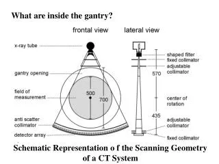
What are inside the gantry? Schematic Representation o f the Scanning Geometry of a CT System
Source- Detector movement Source collimation Detector collimation Generations source detector Advantages Disadvantages No scatter Pencil beam Trans.+Rotates 1st Gen. single single no slow Fan- beamlet Trans.+Rotates Faster than 1G Low efficiency 2nd Gen. yes multiple single High cost and Low efficiency Faster than 2G Fan- beam Rotates together 3rd Gen. many single no Source Rotates only Higher efficiency than 3G Fan- beam high scatter Stationary ring 4th Gen. single no No movement Stationary ring Fan- beam Ultrafast for cardiac high cost 5th Gen. multiple no 3rdGen.+ bed trans. Fan- beam faster 3D imaging higher cost 6th Gen. single many yes Narrow cone- beam 3rdGen.+ bed trans. faster 3D imaging 7th Gen. single Multiple arrays higher cost yes wide cone- beam Relatively slow 3rd Gen. 8th Gen. single no Large 3D FPD
What is displayed in CT images? Water: 0HU Air: -1000HU Typical medical scanner display: [-1024HU,+3071HU], Range: 12 bit per pixel is required in display.
For most of the display device, we can only display 8 bit gray scale. This can only cover a range of 2^8=256 CT number range. Therefore, for a target organ, we need to map the CT numbers into [0,255] gray scale range for observation purpose. A window level and window width are utilized to specify a display. +3071 255 L W 0 -1024
Mass density Mass attenuation coefficient: attenuation per electron or per gram Reminder:
SNR is dependent on dose, as in X-ray. Notice how images become grainier and our ability to see small objects decreases as dose decreases. Next slides discuss analysis of SNR in CT. We will see some similarities with X-ray. But we also see some important differences. Krestel- Imaging Systems for Medical Diagnosis
CT SNR In CT, the recon algorithm calculates the of each pixel. x-ray = No e -∫ dz recorder intensity For each point along a projection g(R), the detector calculates a line integral. n0=Incoming photon density X-ray Source of area A (x,y) ith line integral Detector Ni
Ni = n0 A exp ∫i - dl = N0 exp ∫i - dl where A is area of detector and N0 = n0 A The calculated line integral is ∫i dl = ln (N0/Ni) Mean = ≈ ln (N0/Ni) 2(measured variance) ≈ 1/Ni Now we use these line integrals to form the projections g(R). These projections are processed with convolution back projection to make the image. SNR = C / End Goal
Discrete Backprojection over M projections M • (x,y) = ∑ g(R) * c(R) * (R-R’) ∆ i = 1 add projections convolution back projection where R’ = r cos ( - f ) π Since ∆ = π/M = M/π ∫ g(R) * c(R)* (R-R’) d 0 We can view this as: û = h(r, f ) ** (r, f) estimate Entire system input image or and recon process desired image
C(p) p0 Recall = M/π ∫ g(R) * c(R)* (R-R') d H(p) = (M/π) (C(r) / |r|) is system impulse response of CT system C(r) is the convolution filter that compensates for the 1/|r| weighting from the back projection operation Let’s get a gain (DC) of 1. Find a C(r) to do this. We can consider C(r) = |r| a rect(r/ 2r0). Find constant a H(0) = (M/π) a a = π/M If we set H(0) = 1, DC gain is 1. Therefore, C(p) = (π/M) |r| rect(p/ 2r0). This makes sense – if we increase the number of angles M, we should attenuate the filter gain to get the same gain.
At this point, we have selected a filter for the convolution-back projection algorithm. It will not change the mean value of the CT image. So we just have to study the noise now. The noise in each line integral is due to differing numbers of photons. The processes creating the difference are independent. - different section of the tube, body paths, detector What does this imply about the noise properties along the projection? The set of projections? What does this say for a plan of attack? What effect does the convolution have on the noise?
Recall π = M/π ∫ g(R) * c(R)* (R-R’) d 0 Then the variance at any pixel π 2 = M/π ∫ g2(R)d(R) * [c2(R)]d 0 variance of any one detector measurement Theorem described further at end of these notes. Assume with n = average number of transmitted photons per unit beam width and h = width of beam convolution
C(p) p0 π 2 = (M/π) (1/ (nh)) ∫ d ∫ c2 (R) dR = M/nh ∫ c2 (R) dR 0 Easier to evaluate in frequency domain. Using Parseval’s Rule ∞ 2 = M/(nh) ∫ |C(r)|2 dr -∞ p/M
The cutoff for our filter C(r) will be matched to the detector width w. Let’s let p0 = K/w where K is a constant Combine all the constants n was defined over a continuous projection Let N = nA = nwh = average number of photons per detector element.
In X-ray, SNR √N For CT, there is an additional penalty. To see this, cut w in ½. What happens to SNR? Why Due to convolution operation Another way of looking at it, there is a penalty for oversampling the center or the Fourier space.
Supplementary Random Process Material The following slides may be interesting to someone who has had some background in random processes. It will show how power spectral density analysis is useful in understanding imaging systems. No exams in the class will cover this material. This material is the foundation for the CT noise derivation. First Order Statistics ( What we have studied) m = E[X] = x 2 = E[(x - x)2] Second Order statistic ( Important if we can’t assume independence) RN (x1 , x2) = E [N(x1) N(x2)]
Given an example random process where N = cos (2π fx + ) f is constant, and is uniformly distributed 0 2π RN (x1 ,x2) = ∫ cos (2π fx1 + ) cos (2π fx2 + ) p() d Use cos (a) cos (b) = 1/2 (cos (a - b) + cos (a + b)) p() = 1/2π RN (x1 ,x2) = 1/2π∫1/2[( cos (2π (fx1 + fx2) + 2 ) + (cos(2π(fx1 – fx2)] d First term integrates to 0 across all = ½ cos(2π(fx1 – fx2)) Sample Problem
Autocorrelation Statistic: RN ( ) If mN (x) = m for all x ( i.e. mean stays constant) and the random process is said to be wide sense stationary, then the autocorrelation statistic, RN(t), depends only on the relative distance between two points ( time points, voxels, etc). RN ( ) is a measure of the information one can deduce about a random process if we know the value of the random process at another location. RN (x1 ,x2) = RN ( ) RN ( ) = E [ N(x) N(x + )] The value of the autocorrelation function at 0 represents average power of the random process. This is helpful in measuring noise power. RN (0) = E [ N2 (x)] Measure of average power of random process
Frequency Domain Expression for Random Process • Power spectral density of a Random Process N • We can’t take a meaningful Fourier transform of a random process. But a Fourier transform of RN(t) gives us its power spectrum. This is an indication of where the random processes power resides as a function of frequency. • SN (f) = ∫ RN ( ) e -i 2π f d • RN ( ) = F-1{SN (f)} • = ∫ SN (f) e i 2π xf df • ∞ • E [N2 (x)] = Rx (0) = ∫ SN (f) df • -∞ • How do statistics change after random process is operated by a linear system? N Y H
RY,N ( ) = E [Y(x + ) N(x)] = E [N(x) ∫ N(x + - ) h() d] ∞ = ∫ E [N(x) N(x + - )] h() d -∞ ∞ = ∫ RN ( - ) h() d -∞ = RN ( ) * h ( ) Cross-Correlation What about the autocorrelation of the output Y? That is RY ( ) . ∞ ∞ E [Y(x) Y(x + )] = E [ ∫ h() N(x - ) d • ∫ h() N(x + - ) d ] -∞ -∞ But h(), h() are deterministic. ∞ = ∫ h() h() E[N(x - ) N(x + - )] d d -∞
∞ ∫ h() h() RN ( + - ) d d -∞ ∞ ∫ h()• [h() * RN ( + )] d -∞ RN ( ) = h(-) * h( ) * RN ( ) h(-) H (-f) if real h( ) H(-f) = H*(f) Sy(f) = H*(f)• H(f) • Sx(f) Sy(f) = |H(f)|2 • Sx(f) Average power Ry(0) = ∫ |H(f)|2 •Sx(f) df