Regression as Moment Structure
250 likes | 391 Views
This article explores the moment structure of regression equations, detailing how observable variables relate through regression and moment equations. It discusses parameter estimation methods, particularly in the context of measurement errors affecting the reliability of estimates. We provide sample calculations and data analysis using factor analysis as an example, highlighting issues such as bias in estimates when measurement errors are present. The methods described are applicable in various fields requiring statistical analysis, offering insights into improving regression model accuracy.

Regression as Moment Structure
E N D
Presentation Transcript
Regression Equation Y = b X + v Observable Variables Y z = X Moment matrix sYY sYX S = sYX sXX Moment structure S = S(q) b2sXX +svv bsXX S = bsXXsXX Parameter vector q = (b, sXX, svv )’
Sample: z1, z2, ..., zn n iid • Sample Moments • S = n-1S zi zi’ • syy syx • S = • syx sxx • Fitting S to S = S(q) • Estimator q S close to S = S(q) • 3 moment equations • syy= b2sXX +svv • syx= bsXX • sxx= sXX • with 3 (unknown) parameters • Parameter estimates • q = (syx/sxx, sXX, syy - (b )2sXX )’ ^ ^ ^ ^ b is the same as the usual OLS estimate of b ! ^ ^
Regression Equation Y = b x + v X = x + u Observable Variables Y z = X Moment structure S = S(q) b2sXX +svv bsXX S = bsXXsXX + suu Parameter vector q = (b, sXX, svv , suu )’ new parameter
Sample: z1, z2, ..., zn n iid • Sample Moments • S := n-1zi zi’ • syy syx • S = • syx sxx • Fitting S to S = S(q) • Estimator q = S close to S = S(q ) • 3 moment equations • syy= b2sxx +svv • syx= bsxx • sxx= sxx + suu • with 4 (unknown) parameters • Parameter estimates • q = ?? ^ ^ ^ ^ b is the same as the usual OLS estimate of b ! ^
The effect of measurement error in regression v Y b x X u Y = b (X -u)+ v = bX + (v - bu) = cX + w, where w = v - bu Note that w is correlated with X, unless u or b equals zero So, the classical LS estimate b of b is neither ubiased, neither consistent. In fact, b ---> sYX/sXX = b (sxx/sXX )= kb k is the so called Fiability coefficient (reliability of X). Since 0 k 1 b suffers from downward bias
In multiple regression Regression Equation Y = b1x1 + b2x2...+ b pxp+ v Xk = xk + uk Observable Variables b = SXX-1SXY does not converge to b b* := (SXX - Quu)-1 SXY Examples with EQS of regression with error in variables Using suplementary information to assessing the magnitude of variances of errors in variables.
Path analysis & covariance structure Example with ROS data
Sample covariance matrix ROS92 ROS93 ROS94 ROS95 ROS92 72.07 ROS93 29.5636.21 ROS94 30.2131.0946.51 ROS95 27.63 24.04 35.19 46.62 Mean: 6.27 7.35 10.02 8.80 n = 70 SEM: bj = ? It is a valid model ? F b1 b2 b3 ROS92 ROS93 ROS94
Calculations b1b2= 29.56 b1b3= 30.21 b2b3= 31.09 b1b2/b1b3 = b2/b3 = 29.56/30.21--> b2 = .978b3 31.09 = b2b3= b3 (.978b3) --> b32= 31.09/.978 b3 = 5.64 In the same way, we obtain b1=5.34 b2=5.52 Model test in this case is CHI2 = 0, df = 0
Fitted Model 1 F 5.34 5.52 5.64 R92 R93 R94 43.34 5.80 14.74 CHI2 = 0, df = 0
/TITLE FACTOR ANALYSIS MODEL (EXAMPLE ROS) /SPECIFICATIONS CAS=70; VAR=4; /LABEL V1=ROS92; V2=ROS93; V3=ROS94; V4=ROS95; /EQUATIONS V1 = *F1 + E1; V2 = *F1 + E2; V3 = *F1 + E3; /VARIANCES F1 = 1.0; E1 TO E3 = *; /COVARIANCES /MATRIX 72.07 29.56 36.21 30.21 31.09 46.51 27.63 24.04 35.19 46.62 /END
ROS92 =V1 = 5.359*F1 + 1.000 E1 .974 5.504 ROS93 =V2 = 5.516*F1 + 1.000 E2 .650 8.482 ROS94 =V3 = 5.637*F1 + 1.000 E3 .753 7.482 VARIANCES OF INDEPENDENT VARIABLES ---------------------------------- E D --- --- E1 -ROS92 43.347*I I 8.205 I I 5.283 I I I I E2 -ROS93 5.789*I I 3.924 I I 1.475 I I I I E3 -ROS94 14.736*I I 4.693 I I 3.140 I I I I
… with the help of EQS RESIDUAL COVARIANCE MATRIX (S-SIGMA) : ROS92 ROS93 ROS94 V 1 V 2 V 3 ROS92 V 1 0.000 ROS93 V 2 0.000 0.000 ROS94 V 3 0.000 0.000 0.000 CHI-SQUARE = 0.000 BASED ON 0 DEGREES OF FREEDOM STANDARDIZED SOLUTION: ROS92 =V1 = .631*F1 + .776 E1 ROS93 =V2 = .917*F1 + .400 E2 ROS94 =V3 = .827*F1 + .563 E3
one - factor four- indicators model F * * * * R92 R93 R94 R95 * * * * CHI2 = ?, df = ? p-value = ?
… with the help of EQS /TITLE FACTOR ANALYSIS MODEL (EXAMPLE ROS) ! This line is not read /SPECIFICATIONS CAS=70; VAR=4; /LABEL V1=ROS92; V2=ROS93; V3=ROS94; V4=ROS95; /EQUATIONS V1 = *F1 + E1; V2 = *F1 + E2; V3 = *F1 + E3; V4 = *F1 + E4; /VARIANCES F1 = 1.0; E1 TO E4 = *; /COVARIANCES /MATRIX 72.07 29.56 36.21 30.21 31.09 46.51 27.63 24.04 35.19 46.62 /END
… with the help of EQS ROS92 =V1 = 4.998*F1 + 1.000 E1 .966 5.175 ROS93 =V2 = 4.837*F1 + 1.000 E2 .622 7.779 ROS94 =V3 = 6.417*F1 + 1.000 E3 .653 9.833 ROS95 =V4 = 5.393*F1 + 1.000 E4 .710 7.590 VARIANCES OF INDEPENDENT VARIABLES ---------------------------------- E D --- --- E1 -ROS92 47.090*I I 8.437 I I 5.581 I I I I E2 -ROS93 12.810*I I 2.775 I I 4.616 I I I I E3 -ROS94 5.332*I I 3.017 I I 1.767 I I I I E4 -ROS95 17.536*I I 3.682 I I 4.763 I I
Fitted Model F 4.84 6.42 5.40 4.99 R92 R93 R94 R95 47.10 12.81 5.33 17.54 CHI2 = 6.27, df = 2 p-value = .043
/TITLE FACTOR ANALYSIS MODEL (EXAMPLE ROS) /SPECIFICATIONS CAS=70; VAR=4; /LABEL V1=ROS92; V2=ROS93; V3=ROS94; V4=ROS95; /EQUATIONS V1 = *F1 + E1; V2 = *F1 + E2; V3 = *F1 + E3; V4 = *F1 + E4; /VARIANCES F1 = 1.0; E1 TO E4 = *; /COVARIANCES /CONSTRAINTS (V1,F1)=(V2,F1)=(V3,F1)=(V4,F1); /MATRIX 72.07 29.56 36.21 30.21 31.09 46.51 27.63 24.04 35.19 46.62 /END
… estimation results ROS92 =V1 = 5.521*F1 + 1.000 E1 .528 10.450 ROS93 =V2 = 5.521*F1 + 1.000 E2 .528 10.450 ROS94 =V3 = 5.521*F1 + 1.000 E3 .528 10.450 ROS95 =V4 = 5.521*F1 + 1.000 E4 .528 10.450 CHI-SQUARE = 12.425 BASED ON 5 DEGREES OF FREEDOM PROBABILITY VALUE FOR THE CHI-SQUARE STATISTIC IS 0.02941
... EQS use an iterative optimization method ITERATIVE SUMMARY PARAMETER ITERATION ABS CHANGE ALPHA FUNCTION 1 21.878996 1.00000 1.39447 2 5.741889 1.00000 0.43985 3 2.309283 1.00000 0.19638 4 0.477505 1.00000 0.18079 5 0.147232 1.00000 0.18014 6 0.056361 1.00000 0.18008 7 0.014530 1.00000 0.18007 8 0.005784 1.00000 0.18007 9 0.001423 1.00000 0.18007 10 0.000598 1.00000 0.18007
Exercise: a) Write the covariance structure for the one - factor four- indicators modelb) From the ML estimates of this model, shown in previous slides, compute the fitted covariance matrix.c) In relation with b), compute the residual covariance matrix Note: For c), use the following sample moments: ROS92 ROS93 ROS94 ROS95 ROS92 72.07 ROS93 29.5636.21 ROS94 30.2131.0946.51 ROS95 27.63 24.04 35.19 46.62 Mean: 6.27 7.35 10.02 8.80 n = 70
one - factor four- indicators model with means F 1 * * * * * * * * R92 R93 R94 R95 * * * * CHI2 = ?, df = ? p-value = ?
/TITLE FACTOR ANALYSIS MODEL (EXAMPLE ROS data) /SPECIFICATIONS CAS=70; VAR=4; ANALYSIS = MOMENT; /LABEL V1=ROS92; V2=ROS93; V3=ROS94; V4=ROS95; /EQUATIONS V1 = *V999+ *F1 + E1; V2 = *V999+ *F1 + E2; V3 = *V999+ *F1 + E3; V4 = *V999+ *F1 + E4; /VARIANCES F1 = 1.0; E1 TO E4 = *; /COVARIANCES /CONSTRAINTS ! (V1,F1)=(V2,F1)=(V3,F1)=(V4,F1); /MATRIX 72.07 29.56 36.21 30.21 31.09 46.51 27.63 24.04 35.19 46.62 /MEANS 6.27 7.35 10.02 8.80 /END
ROS92 =V1 = 6.270*V999 + 4.998*F1 + 1.000 E1 1.022 .966 6.135 5.175 ROS93 =V2 = 7.350*V999 + 4.837*F1 + 1.000 E2 .724 .622 10.146 7.779 ROS94 =V3 = 10.020*V999 + 6.417*F1 + 1.000 E3 .821 .653 12.204 9.833 ROS95 =V4 = 8.800*V999 + 5.393*F1 + 1.000 E4 .822 .710 10.706 7.591 VARIANCES OF INDEPENDENT VARIABLES ---------------------------------- E D --- --- E1 -ROS92 47.092*I I 8.437 I I 5.582 I I I I E2 -ROS93 12.810*I I 2.775 I I 4.616 I I I I E3 -ROS94 5.332*I I 3.017 I I 1.767 I I I I E4 -ROS95 17.535*I I 3.682 I I 4.763 I I