Download
1 / 64
640 likes | 657 Views
This meeting introduces the fascinating integration of quantum mechanics principles with NMR technology. Topics covered include Zeeman interaction, chemical shift, spin-spin interactions, and the spin Hamiltonian hypothesis. Explore the complexities of nuclear spin interactions and the underlying physics of angular momentum and magnetic moments. Gain insights into the interplay between magnetic fields and molecules, illustrated by the chemical shift phenomenon. Join us in Khajuraho, India on 16-21 December 2018 to delve into the fundamental concepts bridging NMR and biology.

E N D
4th NMR Meets Biology Meeting NMR introduction:Quantum mechanics meets NMR Konstantin Ivanov (Novosibirsk, Russia) Part 1: NMR interactions Part 2: Basics of spin dynamics Khajuraho, India, 16-21 December 2018
Outline, part 1 • Zeeman interaction • Chemical shift, chemical shift anisotropy; • Spin-spin interactions: dipolar coupling and scalar coupling; • Quadrupolar interaction.
Spin Hamiltonian • In quantum mechanics, we need to solve the Schrödinger equation for ψ or the Liouville-von Neumann equation for ρ • Generally, we need to write down and solve the following equation: Here ψ is the w.f. of the entire system of electrons and nuclei. This equation is virtually impossible to solve. • Solution is provided by the spin Hamiltonian hypothesis: • We limit ourselves to only nuclear spin degrees of freedom, which are decoupled from other degrees of freedom. • Key question: how can we write down the spin Hamiltonian? • In most cases, one can introduce s.H. by separating timescales of electronic and nuclear motions and by keeping in mind that nuclear spin energies are small
Nuclear spin interactions Interactions Electric Magnetic Zeeman interaction Quadrupolar coupling, I>½ Spin-spin interactions, J and D
Angular momentum and magnetic moment • In NMR we deal with spin magnetism. What is ‘spin’? • Charged nucleus (or electron) is spinning: there is angular momentum (spin) and magnetic moment attention: this is a simple view, which is not (entirely) correct The electric current for a charged particle moving around The magnetic moment is q So, μ is proportional to a.m.; when a.m. is measured in ħ units Is it entirely correct? The idea of a very small particle turning around is anyway a simplification…
Angular momentum and magnetic moment So, μ is proportional to a.m.; when a.m. is measured in ħ units Quantum mechanics: this is not entirely correct We are wrong by the g-factor! g=2 for an elementary spin-½ particle (Dirac) How about nuclear spins? Proton g-factor is significantly larger than 2, neutron has magnetic moment Relation between µ and I: q γ-ratio, gyromagnetic ratio
Zeeman interaction • Particles with I≠0 have magnetic moment and interact with external magnetic fields. The energy associated with this interaction is equal to • The field can be static (along Z) or oscillating (along X/Y) • Motion in the static field: precession of µ at the frequency ω=|γ|B • Direction of precession depends on the sign of γ. • Motion in the oscillating transverse field: spin nutation once the resonance condition is fulfilled • The resonance frequency is determined by γ
Chemical shift • The simple expression is (completely) correct only for a nucleus in vacuum • In molecules, electrons change the local field experienced by nuclei: Zeeman interaction is modified • This is a two-stage process: • the external B0 field induces currents in the electronic cloud • when the electrons move, they change the magnetic field at the location of the nucleus: B0→Bloc=B0+Bind • The Bind field is opposite in direction to B0: the field is “shielded” by the electrons • There are two contributions to Bind (having similar magnitude but opposite signs) • circulation of electrons in the ground state (diamagnetic) • involvement of electrons in the excited state (paramagnetic) electrons (shielding) B0 Bind nucleus
Chemical shift • The induced field is always proportional to the B0 field, therefore • The resonance frequency becomes • The new parameter, δ (or σ), is called chemical shift: its precise value depends on the chemical environment of a nucleus (electron density, electronegativity of neighboring atoms, etc.). • Thus, chemical shift is a very important source of information about molecular structure • Chemical shift referencing: • Chemical shift is usually small, so it is measured in ppm’s of ωref • Protons have a spread of δ-values of several ppm; other nuclei have a much wide range of δ-values B0 Bind ωref is the NMR frequency of a standard reference compound (e.g., TMS)
Chemical shift tensor • For a shape asymmetric molecule, the Bind and Bloc fields depend on the orientation • The precise value of Bind depends on the orientation. Mathematically, this effect can be described by introducing the chemical shift tensor • Hence, the induced field becomes: • At high-fields, only the z-component is of importance The Bind value is different in these two cases B0 B0 Bind Bind
Chemical shift tensor, continued • The position of the NMR line is given by δzz, which is different for different orientations of the molecule • In isotropic liquids, the result is simple: fast reorientation of the molecule gives rise to the symmetric CSA tensor. Hence, the isotropic chem. shift is • In solids, for different orientations we obtain a different result. • There are special directions, for which Bind is parallel to B0: principal axes of the δ-tensor. In the principal axes system (PAS) the tensor is diagonal: • When the B0 field is parallel to X,Y,Z of the PAS, the line position is given by δxx, δyy, δzz.
Spin-spin coupling • Two nuclei are two magnetic moments, which interact • There are two contributions: • dipole-dipole interaction, goes through spaces, complete analogue of the classical DDI • scalar coupling, bonding electrons are involved quantum effects • Both contributions can be included in the spin Hamiltonian • The DDI constant depends on the distance between the spins • DDI depends on molecular orientation, given by the vector connecting the spins, J-coupling is isotropic
Dipole-dipole coupling • The DDI Hamiltonian can be written by using tensors: • The D-tensor is a symmetric traceless tensor • For this reason, on average DDI is zero: in isotropic liquids DDI does not change the position of NMR lines • In solids, DDI gives rise to broad lines as it vanishes only at the magic angle. • In high-field approximation (Zeeman term dominates) • The coupling strength is • Some numbers: proton-proton DDI at 1.5 Å is about 35 kHz • DDI scales with γi×γk and decays as 1/r3 Z||B0 Homonuclear case Heteronuclear case
Dipole-dipole coupling • Spectral manifestation of DDI: - In single crystals, DDI gives rise to splitting of the NMR lines. The splitting is given by dik at a specific Θik angle. - In a powder, the splitting is different for different Θikangles (ranging from 0 to π). To calculate the spectrum we need to calculate the splitting for each orientation and weight it with sinΘ. • In some systems, e.g., liquid crystals, partial averaging of DDI takes place. Instead of DDI we deal with RDC (Residual Dipolar Coupling) Such a pattern is termed Pake doublet
H1 vicinal geminal H3 C C H2 Scalar coupling • Indirect coupling, which goes through bonding electrons • Physical origin: • nuclear spins interact with the electrons (hyperfine coupling) • electrons become partly ‘unpaired’ and • start interacting with the other nucleus by creating a small magnetic field • As a result, a nuclear spin-spin coupling emerges • Typically, J-coupling is much smaller than DDI: • For protons the largest coupling is usually the geminalcoupling 2J (15-20 Hz, negative), vicinal coupling 3J is smaller (7 Hz, positive). • For neighboring atoms in the molecule J-couplings are bigger: about 135 Hz for 13C-H, about 50 Hz for 13C-13C • J-couplings are not averaged out by motions. In liquid-state NMR they determine splitting of NMR multiplets
How can we read NMR spectra? • For simplicity, here we discuss only liquid-state NMR. We also ignore any details of the spin dynamicsand use selection rules ΔIz=±1 for NMR transitions (single spin flips/flops) • Hence, we try to construct “stick-spectra”. Interactions, which matter, are chemical shifts and J-couplings. • Algorithm: (1) Different nuclei give signals at very different frequencies because of the large differences in γ’s in experiment we detect separately NMR signals from protons, or carbons, or nitrogens (etc.); (2) Different nuclei of the same kind (e.g., protons) give NMR signals not exactly at the same frequency due to chemical shifts; (3) Lines corresponding to certain nuclei are split due to the presence of other spins ½. Having this strategy, we can draw NMR spectra
Simplifications • (1) Spins will be considered weakly coupled: for each pair of non-equivalents spins difference in Zeeman interactions, ωi–ωj, is much larger than the corresponding coupling Jij; • (2) Quantum mechanics (perturbation theory) tells us that we can leave only JijIizIjzterms (secular terms); • (3) Equivalent spins do not interact with each other (in fact, they do, but these couplings cannot be detected). • What do we call equivalent spins: • Same chemical shifts; • Identical couplings to all other nuclei.
NMR NMR spectrum of two weakly coupled spins Without interaction Withinteraction bAbB bAbB nA/2+nB/2 nA/2+nB/2+J/4 4 4 bAaB bAaB 3 3 nA/2–nB/2 nA/2–nB/2–J/4 –nA/2+nB/2 –nA/2+nB/2–J/4 aAbB aAbB 2 2 1 1 –nA/2–nB/2 –nA/2–nB/2+J/4 aAaB aAaB NMR 4 transitions from rules ΔIz=±1; 4 lines because transitions do not overlap 4 transitions from rules ΔIz=±1; 2 lines because transitions overlap
What to do for a larget number of spins? • Each spin ½ splits NMR line in two lines; their intensities are 2 times lower • Coupling to a group of equivalent spins No other spins +1 spin ½ +2 spins ½ To be continued… J J J′ Relative line intensities in the multiplet Pascal’s triangle 1 1 1 1 2 1 1 3 3 1 N=0 1 2 3
Examples: CH3OH and CH3CH2OH 12 12 3 3 NMR spectrum of methanol 1 1 CH3 OH NMR spectrum of ethanol OH CH2 CH3 Intensity of all lines in the multiplet is proportional to the number of spins in the group Splitting is the same for both spins (same J is operative) Distribution of the intensities is given by Pascal’s triangle rules
Quadrupolar coupling • Q.C. is an electric interaction, which is nonetheless included in the nuclear spin Hamiltonian • Origin of Q.C. • A nucleus has electric charges, which interact with external E-fields • Positive electric charge can be distributed non-uniformly • The charge distribution can be decomposed into multipole components (charge q, dipole moment d, quadrupolar moment Q, etc.); the same is true for the field: the potential is given by the potential V0 at the nucleus, its gradient V1, gradient of the gradient V2, etc. • The energy of interaction is the sum of the following components: E0, energy of q in potential V0 E1, energy of din potential V1 E2, energy of Qin potential V2 continued... • Important: nuclei have d=0! Shape of the nucleus, i.e. charge distribution, is related to the value of its spin I: Q=0 for I=0,½. Spin comes into play!
Quadrupolar coupling • Q.C. is of importance for nuclei with I>½ • It comes from interaction of Q with the electric field gradient at the nucleus • E-field gradient is a tensor, V-tensor: • As any other tensor, it has a PAS, in this frame, simply • The interaction of the E-field gradient with Q can be expressed via I • If HQ is much smaller than the Zeeman terms, we can use perturbation theory. First-order Q.C. is • Second-order Q.C. is about
Quadrupolar coupling • From the expression we can see that • Q.C. vanishes for I=0 and I=½ • Orientation dependence is given by Vzz, which is the zz-component of the V-tensor. • The result is different for a single crystal and for a powder sample • The result is also different for half-integer and for integer I • If we include the second-order terms into consideration the result becomes even more complex. • In some cases, when Q is very large, we have to consider this contribution as well.
Quadrupolar coupling, integer spin Single crystal: Just two lines Powder spectra • Each component is broadened, since the splitting is different for different orientations • For axially-symmetric V-tensor Pake pattern is obtained • Otherwise, the pattern is more complex
Quadrupolar coupling, half-integer spin Single crystal: Just two lines Powder spectra • In a powder, the central line remain narrow • Other lines get broadened, like in the previous example
Summary, part 1 • Key NMR interactions are introduced; • We may also need to mention spin-rotation interaction, which is usually (not always) not that important for NMR; • Spectral manifestations of the interactions are discussed.
Outline, part 2 • Notion of spin; • Spin ensembles: density matrix; • Density matrix description of NMR experiments; • Some examples.
Spin: some history • Zeeman effect: lines split in the presence of magnetic field • Normal Zeeman effect (theory by Lorentz): splitting into three components • Atom is a harmonic oscillator, its frequency is • Problem: anomalous Zeeman effect also exists (met even more often)! • A colleague who met me [Pauli] strolling rather aimlessly in the beautiful streets of Copenhagen said to me in a friendly manner, “You look very unhappy”; whereupon I answered fiercely, “How can one look happy when he is thinking about the anomalous Zeeman effect?” k┴Z k||Z In the presence of B0||Z σ+ σ– σ π σ
Spin: some history • Pauli also tried to solve the problem concerning the number of electrons in each electron shell • For a given n we have l from 0 to (n – 1), lz from –l to ln2 states • In reality there are 2n2 electrons in each shell. Why 2 electrons for n=1, 8 electrons for n=2, 18 electrons for n=3? • Pauli’s answer: (1) there is one more quantum number, which can take only two possible values (Zweideutigkeit) (2) there cannot be two electrons in the same state, i.e., with all q. numbers being the same – exclusion principle • Problem: nice answer, which leads to even harder questions: Why is it so? What is the last quantum number? To what degree of freedom does it correspond?
Spin: some history • Uhlenbeck and Goudsmit: particles have “spin”, corresponding to rotation of a particle spinning around its own axis • Spin of the electron is ½: two states +½=“spin-up” and –½=“spin-down” • This isnot fully consistent from what people knew before. However, this is appropriate because spin is a quantum notion (we do not know why!) • (S + L) can to explain the anomalous Zeeman effect (Pauli can be happy ) • Stern-Gerlach experiment • The beam of atoms is deflected by inhomogeneous field • Reason: intrinsic magnetic moment (spin) of particles • The distribution of the μ-vector is not continuous! • Spin is quantized!!!
Spin • Spin of a particle is its intrinsic angular momentum (as if the particle rotates). Honestly, nobody knows where spin comes from. • Spin is a very fundamental concept, which also affects the symmetry of the w.f. of a system of identical particles. Example: Pauli principle. • Spin is a quantum notion: it vanishes if we tend ħ → 0! • Spin operators are introduced in the same way as those for the angular momentum: eigen-states are ; S2=S(S+1), Sz varies from –S to S. commutation rules are • An important difference from angular momentum: spin can be half-integer • Spin operators are (2S+1)*(2S+1) matrices • For S=1/2 such matrices are related to the Pauli matrices
Spin ½ Basis • Spin operator can be written as • Useful relations of the Pauli matrices: • Every 2*2 hermitian matrix is a linear combination of the unity matrix and the Pauli matrices • Rotations (same results as for L): for an infinitely small rotation for a rotation by an arbitrary angle (rotation by 2π changes the sign of ψ!)
Spin ½: rotations • Generally, the rotation operator is • Explicitly, rotations about X,Y,Z • Euler rotations transition from any reference frame to a new frame can be achieved by three elemental rotations • We go from an old x,y,z to new x,y,z: zyz-rotation by α,β,γ • The rotation operator is
Spin evolution • We can write the Schrödinger equation for the spin w.f. • Here the Hamiltonian (operator, which stands for the energy) is a matrix, which acts on the spin w.f.; it includes magnetic interactions • For instance, interaction with external field, spin-spin interactions, etc. • To solve the time-dependent solution we first solve the eigen-problem • Then the solution is • Physical observables are:
Spin Hamiltonian • To calculate what happens to the spin system we need to know the Hamiltonian • Spins are little magnets, μ is proportional to S • Spin interactions coming from μ • Zeeman interaction in molecules this interaction is modified due to shielding of the external field (chemical shift). Generally, C.S. is a tensor • Interaction with time-dependent RF-fields can be treated in the same way • Spin-spin interaction scalardipolar • Quadrupolar interaction
Simple example: spin ½ particle in an external field • The Hamiltonian • Let us calculate the “spin polarization” vector: • General expression for the w.f.: • Calculation result: • What happens to the P-vector? Example: • The time-dependent S.e. gives the following result (Larmor precession):
Ensemble of spins • This is not the end of the story: the w.f. description is often not sufficient • Example: N1 spins in the α-state and N2 spins in the β-state • What is the P-vector in this case? • When spin ½ has a w.f. |P|=1: the spin ensemble does not have a w.f.! • Similar problems arise when a system contains two subsystems: there might be a total w.f. existing, but (sometimes) no w.f. of a subsystem • What should we do if the w.f. does not exist? Can we still evaluate expectation values of interest and describe experiments?
Density matrix • If we have two sub-ensembles, we calculate expectation values for each realization and then perform averaging • From the mathematical point of view: • The new operator is called “density operator” or “density matrix” • The problem is solved: we can calculate expectation values! • Questions: Properties of the d.m.? Time-dependence of d.m.?
Properties of the density matrix • Physical meaning of the elements: Diagonal elements are populations Off-diagonal elements are coherences ρmn (explained later) • The trace of d.m. is equal to 1 • The d.m. is a hermitian matrix: (N2 – 1) independent parameters • When can we still use the w.f. description? • When the w.f. is existing (pure state), we obtain • When this relation does not hold (mixed state), we must not (!) use the w.f. description. Example: ensemble of spins-1/2 at equilibrium In this case ρ2=ρ does not hold
Density matrix of a spin-½ particle • D.m. of a spin ½ particle • The polarization vector components are • Rewriting the d.m.: • The d.m. is expressed via the P-vector and the Pauli matrices • LongitudinalM = Δ(population); transverseM = coherence • Phase of the coherence: direction in the {x,y}-plane β α β α β α β α
Density matrix of a spin-½ particle • D.m. of a spin ½ particle • The polarization vector components are • Rewriting the d.m.: • We can use the operator basis (each matrix is like a basis ket) • The d.m. is a vector in this basis: • It is easy to obtain the equation of motion (comes later)
Two or more spins ½ • The d.m. for two spins can be expressed in terms of product operators • Each product operator is now a 4*4 matrix; likewise, the Hamiltonian is a 4*4 matrix and it is expressed via the product operators • What is the direct product (Kronecker product)? • Example with 2 spins: • Other operators can be constructed in the same way. More spins: use direct products of spin operators
Two spins ½ • Relation between populations/coherences and d.m. elements • SQCs are given by Sx, Sy, SxIz, SyIz, Ix, Iy, SzIx, SzIy • DQCs and ZQCs are given by combinations of SxIx, SyIy, SxIy, SyIx • We can directly measure only transverse magnetization Sx, Sy, Ix, Iy • Other operators cannot be observed directly, but they affect the signal • Coherence order for ρmn: Energy level diagram Density matrix ββ αβ βα αα
How does the d.m. evolve? • The S.e. in the bra and ket representations is • The equation for the d.m. is as follows: Liouville-von Neumann equation • The solution is simple for a time-independent Hamiltonian: • For a time-dependent Hamiltonian we solve the equation numerically in small time steps or use some tricks • The LvN equation is similar to that for the time-derivative of an operator in the Heisenberg representation. However, the sign is “–” and the meaning is different: in the Heisenberg representation the d.m. and w.f are constant
Time-dependence of the d.m. • The LvN equation is simple in the eigen-basis of the Hamiltonian • The solution is also simple: • Eigen-state populations do not evolve (a quantum system stays forever in an eigen-state); off-diagonal elements oscillate at the ωmn frequency (coherence). • Oscillatory evolution comes about when the initial state is a coherent superposition of eigen-states. • Expectation value of an operator evolves as follows: coherences result in “quantum beats”
Precession of spins ½ • The d.m. is • Likewise, the Hamiltonian is: • So, we can define the P-vector and the field-vector • Substitution to the LvN equation: • The commutator term is: • Finally we obtain precession of the P-vector: • Furthermore, all 2-level systems behave this way: precession of the effective spin in an external field in 3D. The prec. frequency is ωpr=|H|/ħ
Magnetic resonance • Let us consider also the B1-field (circular polarization) • The Hamiltonian is • The LvN equation reads • We can define the d.m. in the rotating frame (interaction representation) • Equation for the new d.m. • The result is (still) precession in an effective field
QM description of NMR experiments • We (usually) start with thermally polarized spins: • The same is true in the rotating frame because the d.m. commutes with the rotation operator; the unity operator can be dropped off. • The d.m. evolves under the action of a time-dependent Hamiltonian (pulses, free evolution, MAS) • Solution methods: split the time-axis into small intervals δt, where H≈const • Looks complex, but the idea is simple: each evolution period leads to two multiplications (at the left and at the right) • In many cases the solution can only be done numerically • When the Hamiltonian is changed in a periodic way, there are some tricks available (AHT, Floquet theory)
RF-pulses the phase is ϕp the flip angle is φ=ω1τp • What happens to the d.m. (magnetization) when we apply a pulse? • The w.f. and d.m. after the pulse • The action of a strong pulse is equivalent to a rotation (we assume that only the B1-term is relevant) • A π/2-pulse generates a coherence, a π-pulse inverts the populations τp ω1 t t+τp
“Sandwich relationships” • Is there a simple way to calculate the effect of pulses? • Three cyclically commuting operators: • Example: • The following relation is then true: • A, B, C are like the axis of our 3D-space; we “rotate” B “around” A by the angle θ. Cyclic permutations provide two more relations • Of course, these rules apply to the spin operators • RF-pulses give x and y-rotations. Free precession gives a z-rotation by a time-dependent angle ωt See M. H. Levitt, “Spin Dynamics”, cyclic commutation