Download
1 / 30
300 likes | 459 Views
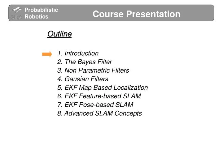
Course Presentation. Outline 1. Introduction 2. The Bayes Filter 3. Non Parametric Filters 4. Gausian Filters 5. EKF Map Based Localization 6. EKF Feature-based SLAM 7. EKF Pose-based SLAM 8. Advanced SLAM Concepts. 1 Introduction. What is Probabilistic Robotics?

E N D
Course Presentation Outline 1. Introduction 2. The Bayes Filter 3. Non Parametric Filters 4. Gausian Filters 5. EKF Map Based Localization 6. EKF Feature-based SLAM 7. EKF Pose-based SLAM 8. Advanced SLAM Concepts
1 Introduction • What is Probabilistic Robotics? • ‘Robotics is the science of perceiving and manipulating the physical world through computer controlled mechanical devices.’ • ‘Probabilistic robotics is a relatively new approach to robotics that pays tribute to the uncertainty in robot perception and action.’ • Sebastian Thrun
Where are the amphoras? Where am I? Robot Localization 1 Introduction ProbabilisticRoboticscourse Localization Mapping
Step: k+2 Step: k+1 The Uncertainty grows without bound. The vehicle gets lost Y X {B} 1 Introduction • Localization: Estimate the position, orientation and velocity of a vehicle • Localization through Dead Reckoning: Step: k
1 Introduction • LocalizationthroughDead-Reckoning: The robot position drifts
1 Introduction • The Mapping Problem • A conventional method for map building is incremental mapping. • Position Reference given by Dead Reckoning Map distorsion • Bad maps Poor localization [Ribas 08]
1 Introduction • The Mapping Problem • A conventional method for map building is incremental mapping. • Position Reference given by Dead ReckoningMap distorsion • Bad mapsPoor localization [Ribas 08]
1 Introduction This is an old problem… Ancient Europe. The Catalan Atlas of 1376.
1 Introduction This is an old problem…
SLAM:Simultaneous Localization And Mapping LocalizationAlgorithms Mapping Algorithms 1 Introduction Map Robot Pose Environment
Step: k+1 Step: k+1 Internal Sensors External Sensors PREDICTION MEASUREMENT Y DATA ASSOCIATION UPDATE X {B} 1 Introduction > Localization Through SLAM: Step: k
1 Introduction > Localization Through SLAM: [Ribas 08]
1.1 Problem Statement “Using sensory information to locate the robot in its environment is the most fundamental problem to providing a mobile robot with autonomous capabilities.” [Cox ’91] • Given • Map of the environment. • Sequence of sensor measurements. • Wanted • Estimate of the robot’s position. • Problem classes • Position tracking (initial pose known) • Global localization (initial pose unknown) • Kidnapped robot problem (recovery)
Y X 1.2 Problem Statement • Pose: • 2D: E(x,y,θ)T • 3D: E(x, y, z,ϕ,θ,φ)T • Environment • Static: only robot pose changes • Dynamic: the robot as well as the pose of other entities change • Localization: • Pasive: Localization module only observes • Active: Robot is guided in a way that minimizes the localization error. x {E} o {G} y y z n {E} x y x Z
DeadReckoning Dead Reckoning: x {E} y z y • [xkykθk] functiongetOdometry() • ΔNL=ReadEncoder(LEFT); • ΔNR=ReadEncoder(RIGHT); • dl = 2 * π * R * ((ΔNL)/ζ) ; • dr= 2 * π* R * ((ΔNR)/ζ) ; • d =(dr+dl)/2; • Δθk=(dr-dl)/w; • θk= θk-1+ Δθk; • xk= xk-1+ (d * cos(θk)); • yk= yk-1+ (d * sin(θk)); • Return [xkykθk] x {B} z
Odometry of the differential drive • [xkykθk] functiongetOdometry() • ΔNL=ReadEncoder(LEFT); • ΔNR=ReadEncoder(RIGHT); • dl = 2 * π * R * ((ΔNL)/ζ) ; • dr= 2 * π* R * ((ΔNR)/ζ) ; • d =(dr+dl)/2; • Δθk=(dr-dl)/w; • θk= θk-1+ Δθk; • xk= xk-1+ (d * cos(θk)); • yk= yk-1+ (d * sin(θk)); • Return [xkykθk] ζ: pulseseach Wheel turn R: Wheel radious
y {E} x x z {B} y 6 DOF Dead Reckoning From Velocity • How can the robot position be defined? • For an 6DOF Mobile Robot (AUV or UAV) Homogeneous Matrix
y {E} x Final configuration 6 DOF Dead Reckoning From Velocity • How can the robot position be defined? • For an 6DOF Mobile Robot (AUV or UAV) Homogeneous Matrix y x y z z x z Position + Roll, Pitch, Yaw attitude X=(x,y,z,ϕ,θ,ψ)
y {E} x z Final configuration 6 DOF Dead Reckoning From Velocity • How can the robot position be defined? • For an 6DOF Mobile Robot (AUV or UAV) Homogeneous Matrix y x z x y z Yaw-Rot(z,ψ) x Position + Roll, Pitch, Yaw attitude y z X=(x,y,z,ϕ,θ,ψ)
y {E} x Final configuration 6 DOF Dead Reckoning From Velocity • How can the robot position be defined? • For an 6DOF Mobile Robot (AUV or UAV) Homogeneous Matrix y x x z z y Yaw-Rot(z,ψ) x z Position + Roll, Pitch, Yaw attitude y z Pitch-Rot(y,θ) X=(x,y,z,ϕ,θ,ψ) x y z
y {E} x x z y Final configuration 6 DOF Dead Reckoning From Velocity • How can the robot position be defined? • For an 6DOF Mobile Robot (AUV or UAV) Homogeneous Matrix y x z Yaw-Rot(z,ψ) x z Position + Roll, Pitch, Yaw attitude y z Pitch-Rot(y,θ) X=(x,y,z,ϕ,θ,ψ) x y z Roll-Rot(x,Φ) x y z
6 DOF Dead Reckoning From Velocity • How can the robot position be defined? • UUV Position & attitude Er=(x, y, z,ϕ, θ, ψ)T • Homogeneous Matrix
Body-fixed u p v w q Y0 X0 r Z0 ro 6 DOF Dead Reckoning From Velocity Position and Euler angles x y Z ϕ Θ ψ • Kinematics Model of an Underwater Robot • Remember Forces and moments X Y Z K M N Lin. and ang. Vel. u (surge) v (sway) w (heave) p (roll) q (pitch) r (yaw) DOF 1 2 3 4 5 6 {B} ηrelative to inertial frame υ,τrelative to fixed-body frame {E} X Y Earth-fixed Z
6 DOF Dead Reckoning From Velocity . • Kinematics Model of an Underwater Robot • Relationship between EηandGυ • Linear Velocity • Angular Velocity y {E} x x z Yaw-Rot(z,ψ) {1} x y z Pitch-Rot(y,θ) x {2} y z Roll-Rot(x,Φ) x y {B} z
6 DOF Dead Reckoning From Velocity . • Kinematics Model of an Underwater Robot • Relationship between Eη andGυ
. Eη 6 DOF Dead Reckoning From Velocity Kinematics Simulation • Kinematics Model of an Underwater Robot x {E} Kinematics y z y x {B} z . Kinematics Inverse Kinematics Bv Bv Eη Direct Kinematics Inverse Kinematics
1.3 Localization Example Example I: Mobile Robot Localization in a Hallway • One dimensional hallway • Indistinguishable doors • Position of doors is known (Map) • Initial position unknown • Initial heading is known • Goal: Find out where the robot is
Same probability of being in any x The Robot senses a door The belief over the position is updated The Robot Moves The belief over the position is updated The Robot senses a door The belief over the position is updated The Robot Moves The belief over the position is updated 1.3 Localization Example • Markov Localization
1.3 Localization Example Robot belief of being at state xt-1 ut State Transition probability 2 4 6 ut ut=6 m, xt-1=5 m ut=4 m, xt-1=5 m ut=2 m, xt-1=5 m xt-1 5 7 9 11 2 4 6 ut=6 m, xt-1=3 m ut ut=4 m, xt-1=3 m ut=2 m, xt-1=3 m xt-1 3 5 7 9
Prior Belief. Prediction of state xt. Measurement probability Robot belief of being at state xt 1.3 Localization Example Robot belief of being at state xt-1 ut State Transition probability 2 ut=2 m, xt-1=5 m 5 7