Download
1 / 50
500 likes | 640 Views
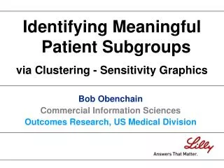
Identifying Meaningful Patient Subgroups via Clustering - Sensitivity Graphics. Bob Obenchain Commercial Information Sciences Outcomes Research, US Medical Division. Rosenbaum PR. Observational Studies, Second Edition. New York: Springer-Verlag. 2002, page 5.

E N D
Identifying Meaningful Patient Subgroups via Clustering - Sensitivity Graphics Bob Obenchain Commercial Information Sciences Outcomes Research, US Medical Division
Rosenbaum PR. Observational Studies, Second Edition. New York: Springer-Verlag. 2002, page 5. In its essence, to “adjust for age” is to compare smokers and nonsmokers of the same age. …differences … in age-adjusted mortality rates cannot be attributed to differences in age. Adjustments of this sort, for age or other variables, are central to the analysis of observational data.
Cochran WG, Cox G.Experimental Designs 1957 • Blocking • Randomization • Replication
Forms of Local Control for Human Studies • Epidemiology (case-control & cohort) studies • Post-stratification and re-weighting in surveys • Stratified, dynamic randomization to improve balance on predictors of outcome • “Full Matching” on Propensity Score estimates • Econometric Instrumental Variables (LATEs) • Marginal Structural Models (InvProbWgt 1/PS) • Unsupervised Propensity Scoring: Nested (Treatment within Cluster) ANOVA …with LOA, LTD and Error components
“Local” Terminology: • Subgroups of Patients • Subclasses… • Strata… • Clusters…
Nested ANOVA Although a NESTED model can be (technically) WRONG, it is sufficiently versatile to almost always be USEFUL as the number of “clusters” increases.
In general, subgroups of patients can be considered meaningful only if patients are much more similar within subgroups than between subgroups.
Notation for Variables y= observed outcome variable(s) x= observed baseline covariate(s) t= observed treatment assignment (usually non-random) z= unobserved explanatory variable(s)
When making head-to-head treatment comparisons, subgroups of patients remain meaningful only if the observed distributions of within subgroup differences in outcome due to treatment also differ among subgroups.
When making head-to-head treatment comparisons, subgroups of patients remain meaningful only if the observed distributions of within subgroup differences in outcome due to treatment also differ among subgroups.
Meaningful subgroups can only contain smaller patient subgroups that are not meaningful. Overshooting!!!
16 Clusters (each containing both treated and untreated patients) in a two dimensional X-space Different Possible LTD Distributions of Y Outcomes will be Illustrated here in the Bottom Half of the Following Slides...
16 Clusters (each containing both treated and untreated patients) in a two dimensional X-space These clusters may NOT be “meaningful” when the resulting distribution of treatment differences in Y looks quite peaked: Main Effect with Little Noise
16 Clusters (each containing both treated and untreated patients) in a two dimensional X-space However, these clusters are “meaningful” when the resulting distribution of treatment differences in Y is different from the corresponding distribution using RANDOM subgroups:
Artificial LTD Distributions from • Random Subgroupings… • Relatively Flat?, Smooth? or Unimodal? • Maximum Uncertainty and Bias because least relevant comparisons are included !!! • LTD Distributions from Subgroups • Relatively Well-Matched in X-space… • Shifted Mean? Skewness? • Distinct Local Modes? • Lower Local Variability? …Meaningful!
16 Clusters (each containing both treated and untreated patients) in a two dimensional X-space These clusters may be meaningful when the distribution of treatment differences in Y looks something like this:
16 Clusters (each containing both treated and untreated patients) in a two dimensional X-space These 7 clusters are meaningful when the distribution of treatment differences reveals a “local mode” attributable to “adjacent” clusters:
16 Clusters (each containing both treated and untreated patients) in a two dimensional X-space Clusters could fail to remain meaningful if the “local mode” in thedistribution of treatment differences corresponds to outcomes from widely dispersed clusters:
Traditional Covariate Adjustment methods used in Randomized Clinical Trials (i.e. Least Square Means) make very strong assumptions: • Their (complex?) parametric models are correct. • Factors should compete for (causal) credit. • Subgroup-based approaches used in Observational Human Studies face “reality”: • (Non-parametric) Nested ANOVA models (treatment within subgroup) are “robust.” • Sometimes, it’s just not possible to make clearly fair comparisons!
What is a Treatment Effect? • Global / Marginal Inference… • Difference of Overall Averages • …one average for each treatment group or a simple “contrast” (single degree-of-freedom) • Local / Conditional Inference… • Distribution of Local Differences • …one treatment difference within each informative subgroup of similar patients
Mortality Rates: Simpson’s Paradox Mild Severe W-Class 1% 6% Local 3% 9% Difference:2% 3% Total 4.4% 3.8% +0.6% Mild Severe Total W-Class 3/327 41/678 44/1005 Local 8/258 3/33 11/291 Total 11/585 44/711 Disease severity is a confounder here in the sense that it is associated with both outcome (mortality) and treatment choice (hospital.)
The “statistical methodology” engine ideal for making fair treatment comparisons is: Cluster Analysis (Unsupervised Learning) plus Nested ANOVA i.e. not Generalized Linear Models and their Nonlinear extensions.
Is there statistical “theory” suggesting use of clustering to identify treatment effects?
Fundamental PS Theorem Joint distribution ofxandtgivenp: Pr( x, t | p ) = Pr( x | p ) Pr( t | x, p ) = Pr( x | p ) Pr(t|x) = Pr( x | p ) timespor(1p) = Pr( x | p ) Pr( t | p ) ...i.e xandtareconditionally independentgiven thepropensity for new, p= Pr(t = 1| x ).
Conditioning (patient matching) on estimated Propensity Scores implies both… Balance: local X-covariate distributions must be the same for both treatments and Imbalance: Unequal local treatment fractions unless Pr( t | p ) = p = 1p= 0.5
Pr( x, t | p ) = Pr( x | p ) Pr( t | p ) The unknown true propensity score (in non-randomized studies) is the “most coarse” possible balancing score. The known X-vector itself is the “most detailed” balancing score… Pr( x, t ) = Pr( x ) Pr( t | x )
Pr( x, t | p ) = Pr( x | p ) Pr( t | p ) The unknown true propensity score (in non-randomized studies) is the “most coarse” possible balancing score. The known X-vector itself is the “most detailed” balancing score… Pr( x, t ) = Pr( x ) Pr( t | x )
Pr( x, t | p ) = Pr( x | p ) Pr( t | p ) The unknown true propensity score (in non-randomized studies) is the “most coarse” possible balancing score. Conditioning upon Cluster Membership is intuitively somewhere between the two PS extremes in the limit as individual clusters become numerous, small and compact… Pr( x, t | C ) Pr( x | C ) Pr( t| x, C ) constant Pr( t | C ) The known X-vector itself is the “most detailed” balancing score… Pr( x, t ) = Pr( x ) Pr( t | x )
Start by Clustering Patients in X-Space 3 clusters 21 clusters Divisive Coefficient = 0.98
In Randomized Experiments, fraction treated (imbalance) will vary from subgroup to subgroup due to: • Bad Luck (Murphy’s Law) • Small Subgroups • In Observational Human Studies, fraction treated (imbalance) varies even more from subgroup to subgroup due to: • 3. Treatment Selection Biases
Nested ANOVA Although a NESTED model can be (technically) WRONG, it is sufficiently versatile to almost always be USEFUL as the number of “clusters” increases.
Nested ANOVA Treatment Difference within ith Cluster: Local Treatment Imbalance!
Local Control: A Subgroup / Sensitivity Graphics approach to Robustness Replace covariate adjustment based upon a global model with inference based upon local clustering (sub-grouping) of patients in X-covariate space. Explore sensitivity by increasing the number of clusters, intentionally over-shooting, then recombining. Also vary distance metric and clustering method while employing computationally intensive algorithms and interactive graphical displays.
Common Threads: • Many possible answers !!! • No single approach nor set of assumptions is clearly most appropriate. Urgent need for “Up Front” Sensitivity Analyses
Survey of 1314 Whickham Women y= 20 year mortality (yes or no) in 1995 follow-up study of a survey made in 1972-1974 x= age decade (20, 30, 40, 50, 60, 70 or 80) at the time of the initial survey t= smoker or non-smoker at the time of the initial survey Appleton DR, French JM, Vanderpump MPJ. “Ignoring a Covariate: An Example of Simpson’s Paradox” Amer. Statist. 1996; 50: 340-341.
20 Year Mortality Rate Difference Overall Mean and +/-Two Sigma Limits for the Distribution of LTD Differences: Mortality Rate of Smokers minus that of Nonsmokers. Number of Clusters
Simpson’s Paradox At Work: Percentage of Smokers by Age Decade …and 20 Year Mortality Percentages for Smokers and Non-Smokers
1.0 0.9 0.8 0.7 0.6 0.5 Cum Prob 0.4 0.3 0.2 0.1 -0.2 -0.1 0 .1 .2 .3 LTD Distribution of Heteroskedastic Estimates… 49 Informative Clusters for 20 Year Mortality of 1314 Wickham Women: Smokers minus Nonsmokers CDF KEY QUESTIONS: • Is this distribution mostly just noise around some central value? • How many local modes might this distribution really have? • Do the Xs predict the most likely LTD for some (or all) patients?
Mixture Joint Density: |12|/ 1 2 3
Future “Needs” • Continuing evolution in methodologies for and attitudes about analyses of non-randomized human studies • Postpone decisions whenever available data are insufficient to provide high confidence • Statistical methods CAN work better-and-better in the dense data limit
References Hansen BB. “Full matching in an observational study of coaching for the SAT.” JASA 2004; 99: 609-618. Fraley C, Raftery AE. “Model based clustering, discriminant analysis and density estimation.”JASA 2002; 97: 611-631. Imbens GW, Angrist JD. “Identification and Estimation of Local Average Treatment Effects.”Econometrica 1994; 62: 467-475. McClellan M, McNeil BJ, Newhouse JP. “Does More Intensive Treatment of Myocardial Infarction in the Elderly Reduce Mortality?: Analysis Using Instrumental Variables.”JAMA 1994; 272: 859-866.
References …concluded McEntegart D. “The Pursuit of Balance Using Stratified and Dynamic Randomization Techniques: An Overview.” Drug Information Journal 2003; 37: 293-308. Obenchain RL. “Unsupervised Propensity Scoring: NN and IV Plots.” 2004 Proceedings of the ASA. Obenchain RL. “Unsupervised and Supervised Propensity Scoring in R: the USPS package” March 2005. http://www.math.iupui.edu/~indyasa/download.htm. Rosenbaum PR, Rubin RB. “The Central Role of the Propensity Score in Observational Studies for Causal Effects.”Biometrika 1983; 70: 41-55. Rosenbaum PR. Observational Studies, Second Edition. 2002. New York: Springer-Verlag.
Current GuidelineInitiatives… • Randomized Clinical Trials • CONSORT: www.consort-statement.org • Observational & Non-randomized Studies • STROBE: www.strobe-statement.org • TREND: www.trend-statement.org
The Propensity Score of a Patient with Baseline Characteristic Vector x : PS = Pr(t |x ) is a vector of conditional probabilities that sum to 1. The length of the PS vector is the total (finite) number of different treatments.
Propensity Scores for only 2 Treatments: t = 1 (new) or 0 (standard) p = Propensity for New Treatment = Pr(t= 1 |X ) = E(t|X) = a scalar valued function ofX only X = vector of baseline covariate values for patient PS = (p, 1p)
0 Y-outcome-difference
0 Y-outcome-difference
0 Y-outcome-difference