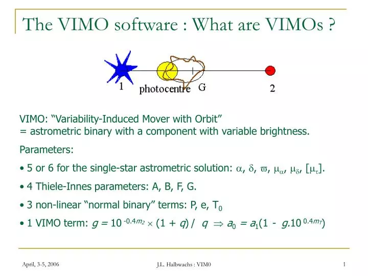

The VIMO software : What are VIMOs ?
E N D
Presentation Transcript
The VIMO software : What are VIMOs ? • VIMO: “Variability-Induced Mover with Orbit” • = astrometric binary with a component with variable brightness. • Parameters: • 5 or 6 for the single-star astrometric solution: , , , , , []. • 4 Thiele-Innes parameters: A, B, F, G. • 3 non-linear “normal binary” terms: P, e, T0 • 1 VIMO term: g= 10 -0.4m2 (1 + q)/ q a0 = a1(1 - g.10 0.4mT) J.L. Halbwachs : VIM0
The VIMO strategy: search of g (1) • g= 10 -0.4m2 (1 + q) / q a0 = a1(1 - g.10 0.4mT) • Minimum g : comes from the minimum variation of a0 for a VIM effect; a0 > c X , a1 = a q / (1+q) • gmin = c X10 -0.4mmin/ [ aMax(1 – 10-0.4m) ] with m = mmin-mMax >0 • Maximum g : m2 > mT gMax = 10-0.4 mmin(1 + qmin) / qmin • • assuming aMax= 50 mas, X = 40 as, c = 1, m = 1 mag, qmin= 0.5, g.10 0.4mmin ranges from 0.00133 up to 3. • For security, aMax = 100 mas, c=1/4 and qmin=0.01 are assumed, leading to gMax/gmin=6 105 when m=1 mag. J.L. Halbwachs : VIM0
The VIMO strategy: search of g (2) Fortunately, the interval of g may be restricted assuming fixed P (ie 100 d), and e (ie 0) and trial values of g, all the other parameters are derived (linear system). When the star is a VIMO, 2(g) is usually varying for g around its actual value new interval : g0/10 – 10 g0 (100 trial values) Having g, we adapt the method of Pourbaix & Jancart (2003) J.L. Halbwachs : VIM0
The VIMO strategy: search of P Assuming e =0 and using trial P and g, we have a system of linear equations. P is then generally corresponding to theminimum of 2(P,g)(Pourbaix & Jancart, DMS-PJ-01, 2003). Otherwise, up to 5 minima of 2(P,g;e=0) are tested. If an acceptable P is still not found, other eccentricities are tried: e=0.7 (6 trial T0) and e=0.9 (8 trial T0) Time-consuming !! J.L. Halbwachs : VIM0
The VIMO strategy: the solution For a minimum of 2(P, e=0), preliminary values of e and T0 are still obtained trying e=0.1 and e=0.5 in place of e=0; having starting values for P ( log P ), g ( log g), e ( -log(-log e)), T0andfor the “linear” parameters,a solution is calculated using the Levenberg-Marquardt method of 2 minimisation. Other minima of 2 are tried until a solution with GOF < 3 is obtained ( risk to keep a local minimum when the orbit is small !) J.L. Halbwachs : VIM0
VIMO simulation: hypotheses • VIMO with large orbits : • a = 50 mas, X = 40 as, • f(log P ;10days < P < 10 years) = Cst, • f(e < 0.9) = Cst, • f(q ; 0.1 < q < 1.2) = Cst ( q = M2/M1, where “1” refers to the variable) • m2-m1= 6.6 log q + m ; f(m) = N (0,1) • photometric variations a0varying a0 2.5X J.L. Halbwachs : VIM0
VIMO simulation: results Solutions for 93 systems/100 <(Psolution– Pactual)/IP> = -0.08 <(esolution– eactual)/Ie> = 0.16 E/I = 1.03 E/I = 1.11 J.L. Halbwachs : VIM0
The Goodness-Of-Fit problem • F2 (Hipparcos, vol 1, 112) : inadequate since the model is not linear. • Degrees of freedom derived by Fourier transform (Pourbaix DMS-DP-02, 2005) : e and T0 exchanged with (many) linear terms. With large VIMO orbits : <F2> = 0.12, = 1.4 <GOFF> = 2.2, = 1.7 both N (0,1) J.L. Halbwachs : VIM0
Still to be done .. • Adaptation of the software to small orbits (trying other minima of 2). • To compute faster ! current rate : 10 stars/hour (PC). The number of trial values could be reduced. - False candidates must be discarded : acceleration+VIM solutions must be searched (3 VIMacc parameters). J.L. Halbwachs : VIM0
Searching VIMO in Hipparcos .. • Hipparcos published archive: • Stochastic solutions. • Epoch Photometry Annex: H-mag for each transit • Intermediate Astrometric Data: Average abscissae for 1 orbit of the satellite (10 h) !!! • no short period variable, no variable with fast variation (WW UMa, BY Dra, flare stars ..) • no nearby stars • no astrometric orbit with P 3 years, • .. but an opportunity to see the difficulties with real data J.L. Halbwachs : VIM0
Is HIP 88848 a VIMO (1) ? single star model: 2 =280, F2=17.8 (NDAC) 1st VIMO solution : 2 = 26.5, F2=-0.17 P = (1595 1574) d g = (4.3 2.1) 10-4 A SB+AB (Feckel,..,Jancart & Pourbaix 2005) : P = 2092 days J.L. Halbwachs : VIM0
HIP 88848 assuming SB elements New VIMO solution starting from the SB elements: With NDAC data: 2 = 26.4, F2=-0.18, GOFF=1.02 P = (21473855) d g = (3.72.7) 10-4 a1 = 91 mas (instead of 48..) NOT a VIMO !!! J.L. Halbwachs : VIM0
Searching g in stochastic stars “Stochastic stars” = single stars generated with X much larger than assumed in the VIMO calculation. J.L. Halbwachs : VIM0
Conclusion • A prototype software • providing reliable solutions when variability induces important astrometric effects, • but inept results otherwise ... • • The software must still be adapted to small orbits • VIMO solutions • must be searched only when no “normal” solution can be found • must be kept only when the estimated errors are reasonable J.L. Halbwachs : VIM0
Searching VIMO in Hipparcos .. J.L. Halbwachs : VIM0