Download

1 / 24
370 likes | 1.7k Views
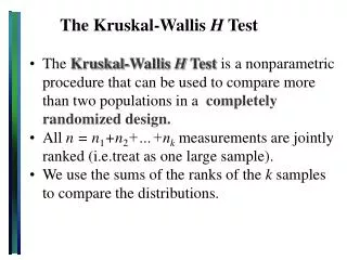
The Kruskal-Wallis H Test. Sporiš Goran, PhD. http://kif.hr/predmet/mki http://www.science4performance.com/. The Kruskal-Wallis H Test. The Kruskal-Wallis H Test is a nonparametric procedure that can be used to compare more than two populations in a completely randomized design.

E N D
The Kruskal-Wallis H Test Sporiš Goran, PhD. http://kif.hr/predmet/mki http://www.science4performance.com/
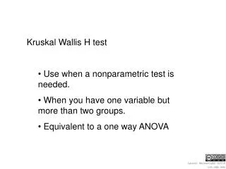
The Kruskal-Wallis H Test • The Kruskal-Wallis H Test is a nonparametric procedure that can be used to compare more than two populations in a completely randomized design. • All n = n1+n2+…+nkmeasurements are jointly ranked (i.e.treat as one large sample). • We use the sums of the ranks of the k samples to compare the distributions.
The Kruskal-Wallis H Test • Rank the total measurements in all k samples from 1 to n. Tied observations are assigned average of the ranks they would have gotten if not tied. • Calculate • Ti = rank sum for the ith sample i = 1, 2,…,k • And the test statistic
The Kruskal-Wallis H Test H0: the k distributions are identical versus Ha: at least one distribution is different Test statistic: Kruskal-Wallis H When H0 is true,the test statistic H has an approximate chi-square distribution with df = k-1. Use a right-tailed rejection region or p-value based on the Chi-square distribution.
1 2 3 4 65 75 59 94 87 69 78 89 73 83 67 80 79 81 62 88 Example Four groups of students were randomly assigned to be taught with four different techniques, and their achievement test scores were recorded. Are the distributions of test scores the same, or do they differ in location?
1 2 3 4 (3) 65 (7) 75 59 (1) (16) 94 87 (13) (5) 69 78 (8) 89 (15) (6) 73 83 (12) 67 (4) (10) 80 (9) 79 81 (11) 62 (2) (14) 88 Ti 31 35 15 55 Teaching Methods Rank the 16 measurements from 1 to 16, and calculate the four rank sums. H0: the distributions of scores are the same Ha: the distributions differ in location
Teaching Methods H0: the distributions of scores are the same Ha: the distributions differ in location Reject H0. There is sufficient evidence to indicate that there is a difference in test scores for the four teaching techniques. Rejection region: For a right-tailed chi-square test with a = .05 and df = 4-1 =3, reject H0 if H 7.81.
Key Concepts I. Nonparametric Methods These methods can be used when the data cannot be measured on a quantitative scale, or when • The numerical scale of measurement is arbitrarily set by the researcher, or when • The parametric assumptions such as normality or constant variance are seriously violated.
Key Concepts Kruskal-Wallis H Test: Completely Randomized Design 1. Jointly rank all the observations in the k samples (treat as one large sample of size n say). Calculate the rank sums, Ti= rank sum of sample i, and the test statistic 2. If the null hypothesis of equality of distributions is false, H will be unusually large, resulting in a one-tailed test. 3. For sample sizes of five or greater, the rejection region for H is based on the chi-square distribution with (k- 1) degrees of freedom.
Testing for trends: the Jonckheere-Terpstra test This test looks at the differences between the medians of the groups, just as the Kruskall-Wallis test does. Additionally, it includes information about whether the medians are ordered. In our example, we predict an order for the number of sperms in the 4 groups, indeed: no meal > 1 meal > 4 meals > 7 meals In the coding variable, we have already encoded the order which we expect (1>2>3>4)
If you have J-T in your version of SPSS, it would look like this Output of the J-T test Z-score = (912-1200)/116.33=-2.476 J-T test should always be 1-tailed (since we have a directed hypo!) We compare -2.47 against 1.65 which is the z-value for an -level of 5% for a 1- tailed test. Since 2.47>1.65 the result is significant. The negative sign means that medians are in descending order (a positive sign would have meant ascending order).
Differences between several related groups: Friedman's ANOVA • Friedman's ANOVA is the non-parametric analogue to a repeated measure ANOVA (see chapter 11) where the same subjects have been subjected to various conditions. • Example here: Testing the effect of a new diet called 'Andikins diet' on n=10 women. Their weight (in kg) was tested 3 times: • Start • Month 1 • Month 2 • Would they loose weight in the course of the diet?
Theory of Friedman's ANOVA Always the 3 scores are compared: The smallest one gets 1, the next 2, and the biggest one 3. • Subject's weight on each of the 3 dates is listed in a separate column. Then ranks for the 3 dates are determined and listed in separate columns. • Then, the ranks are summed up for each Condition (Ri) Diet data with ranks
The Test statistic Fr From the sum of ranks for each group, the test statistic Fr is derived: k Fr = 12/Nk (k+1) Σi=1R2i - 3N(k+1) = (12/(10x3)(3+1)) (192 + 202 + 212)) – (3x10)(3+1) =12/120 (361+400+441) – 120 =0.1 (1202) – 120 =120.2 - 120 = 0.2
Data Input and provisional analysis (using) diet.sav Data sheet First, test for normality: Analyze Descriptive Statistics Explore, tick 'Normality plots with tests' in the 'Plots' window In the Shapiro-Wilk test (which is more accurate than the K-S Test, two groups (Start, 1 month) show non-normal distributions. This violation of a parametric constraint justifies the choice of a non-para-metric test.
Running Friedman's ANOVA Analyze Non-parametric Tests K Related Samples... If you have 'Exact', tick 'Exact and limit calculation time to 5 minutes. Other options Other options Exact... Request everything there is - it is not much...
Other options • Kendall's W: Similar to Friedman's ANOVA, but looks specifically at agreement between raters. For example: to what extent (from 0-1) women rate Justin Timberlake, David Beckham, or Tony Blair on their attractiveness. This is like a correlation coefficient. • Cochran's Q: This is an extension of NcNemar's test. It is like a Friedman's test for dichotomous data. For example, if women should judge whether they would like to kiss Justin Timberlake, David Beckham, or Tony Blair and they could only answer: Yes or No.
Output from Friedman's ANOVA The F-Statistics is called Chi-Square, here. It has df=2 (k-1, where k is the # of groups). The statistics is n.s.
Posthoc tests for Friedman's ANOVAWilcoxon signed-rank tests but correcting for the numbers of tests we do, here = .05/3=.0167. Analyze Nonparametric Tests 2-Related Tests, tick 'Wilcoxon', specify the 3 pairs of groups Mean ranks and sum of ranks for all 3 comparisons So, actually, we do not have to calculate any further... All comparisons are ns, as expected from the overall ns effect.
Posthoc tests for Friedman's ANOVA- calculation by hand We take the difference between the mean ranks of the different groups and compare them to a value based on the value of z (corrected for the # of comparions) and a constant based on the total sample size (n=10) and the # of conditions (k=3) Ru - Rvzk(k-1) k(k+1)/6N zk(k-1) = .05/3(3-1) = .00833 If the difference is significant, it should have a higher value than the value of z for which only .00833 other values of z are bigger. As before, we look in the Appendix A.1 under the column Smaller Portion. The number corresponding to .00833 is the critical value: it is between 2.39 and 2.4. k(k-1) = 3 (3-1) = 6
Calculating the critical differences Critical difference = zk(k-1) k(k+1)/6N crit. Diff = 2.4 (3(3+1)/6x10 crit. Diff = 2.4 12/60 crit. Diff = 2.4 0.2 crit. Diff = 1.07 If the differences between mean ranks are the critical difference 1.07, then that difference is significant.
Calculating the differences between mean ranks for diet data None of the differences is the critical difference 1.07, hence none of the comparisons is significant.
Calculating the effect size Again, we will only calculate the effect sizes for single comparisons: • r = z • 2n • rStart – 1 month = -0.051/ = -.01 • rStart – 2 months = -0.255/0 = -.06 • r1 month – 2 months = -0.153/0 =-.03 Tiny effects Tiny effects Tiny effects
Reporting the results of Friedman's ANOVA (Field_2005_566) „The weight of participants did not significantly change over the 2 months of the diet (2(2) = 0.20, p > .05). Wilcoxon tests were used to follow up on this finding. A Bonferroni correction was applied and so all effects are reported at a .0167 level of significance. It appeared that weight didn't significantly change from the start of the diet to 1 month, T=27, r=-.01, from the start of the diet to 2 months, T=25, r=-.06, or from 1 month to 2 months, T=26,r=-0.3. We can conclude that the Andikinds diet (...) is a complete failure.“