Describing algorithms in pseudo code
Describing algorithms in pseudo code. To describe algorithms we need a language which is: less formal than programming languages (implementation details are of no interest in algorithm analysis); easy to read for a human reader.

Describing algorithms in pseudo code
E N D
Presentation Transcript
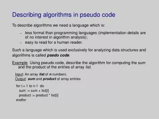
Describing algorithms in pseudo code To describe algorithms we need a language which is: • less formal than programming languages (implementation details are of no interest in algorithm analysis); • easy to read for a human reader. Such a language which is used exclusively for analyzing data structures and algorithms is called psedo code. Example Using pseudo code, describe the algorithm for computing the sum and the product of the entries of array list. Input: An array list of n numbers. Output: sum and product of array entries for i:= 1 to n-1 do sum := sum + list[i] product := product * list[i] endfor
Pseudo code: basic notation 1. We will use := for the assignment operator (<-- in the book), and = for the equality relationship. 2. Method signatures will be written as follows: Algorithm name ({parameter list}) 3. Programming constructs will be described as follows: • decision structures: if ... then ... else ... • while loops: while ... do {body of the loop} • repeat loops: repeat {body of the loop} until ... • for loops: for ... do {body of the loop} • array indexing: A[i] 4. Method calls: Method name ({argument list}) 5. Return from methods: return value
More examples on describing and analyzing algorithms: the sorting problem The objective of the sorting problem: rearrange a given sequence of items so that an item and its successor satisfy a prescribed ordering relationship. To define an instance of a sorting problem, we must specify: • the type of the sequence; • the number of items to be sorted; • the ordering relationship. Consider the following instance of the sorting problem: an array of integers, A, containing N items is to be sorted in ascending order. We will review three algorithms for sorting known as elementary sorts: • the bubble sort algorithm, • the selection sort algorithm, and • the insertion sort algorithm.
Bubble sort. The idea: Make repeated passes through a list of items, exchanging adjacent items if necessary. At each pass, the largest unsorted item will be pushed in its proper place. Stop when no more exchanges were performed during the last pass. The algorithm: Input: An array A storing N items Output: A sorted in ascending order Algorithm Bubble_Sort (A, N): for i := 1 to N-1 do { for j := 0 to N-i do { if A[j] > A[j+1] temp := A[j], A[j] := A[j+1], A[j+1] := temp } }
Run time efficiency of bubble sort Two operations affect the run time efficiency of the bubble sort the most: • the comparison operation in the inner loop, and • the exchange operation also in the inner loop. Therefore, we must say how efficient the bubble sort is w.r.t. each of the two operations. • Efficiency w.r.t. the number of comparisons: • during the first iteration of the outer loop, in the inner loop (N - 1 comparisons); • during the second iteration of the outer loop: (N - 2 comparisons); • ......... • during the (N - 1)-th iteration of the outer loop: 1 comparison. Total number of comparisons: (N - 1) + (N - 2) + ... + 2 + 1 = (N * (N - 1)) / 2 = (N^2 - N) / 2 < N^2 Bubble sort is O(N^2) algorithm w.r.t. the number of comparisons.
Run time efficiency of bubble sort (cont.) • Efficiency w.r.t. the number of exchanges: • during the first iteration of the outer loop, in the inner loop: at most (N - 1 exchanges); • during the second iteration of the outer loop: at most (N - 2 exchanges); • ......... • during the (N - 1)-th iteration of the outer loop: at most 1 exchange. Total number of exchanges: (N - 1) + (N - 2) + ... + 2 + 1 = (N * (N - 1)) / 2 = (N^2 - N) / 2 < N^2 Bubble sort is O(N^2) algorithm w.r.t. the number of exchanges. Note that only one pass through the inner loop is required if the list is already sorted. That is, bubble sort is sensitive to the input, and in the best case (for sorted lists) it is O(N) algorithm wrt the number of comparisons, and O(1) wrt the number of exchanges.
An example implementation of bubble sort interface AnyType { public boolean isBetterThan(AnyType datum); } class IntegerType implements AnyType { private int number; IntegerType() {number = 0; } IntegerType(int i) {number = i; } public boolean isBetterThan(AnyType datum) { return (this.number > ((IntegerType)datum).number); } public int toInteger() {return number; } } class StringType implements AnyType { private String word; StringType(){word = "";} StringType(String s){word = s;} public boolean isBetterThan(AnyType datum) { return (this.word.compareTo(((StringType)datum).word) > 0); } public String toString() { return word; } }
Implementation of bubble sort (cont) class BubbleSort { public static void bubbleSort(AnyType[] array) { AnyType temp; int numberOfItems = array.length; boolean cont = true; for (int pass=1; pass != numberOfItems; pass++) { if (cont) { for (int index=0; index != numberOfItems-pass; index++) { cont = false; if (array[index].isBetterThan(array[index+1])) { temp = array[index]; array[index] = array[index+1]; array[index+1] = temp; cont = true; } // end inner if } // end inner for } else break; // end outer if } } }
Selection sort. The idea: Find the smallest element in the array and exchange it with the element in the first position. Then, find the second smallest element and exchange it with the element in the second position, and so on until the entire array is sorted. The algorithm: Input: An array A storing N items Output: A sorted in ascending order Algorithm Selection_Sort (A, N): for i:= 1 to N-1 do { min := i for j:= i+1 to N do if A[j] < A[min] then min := j temp := A[min], A[min] := A[i], A[i] := temp }
Run time efficiency of selection sort Two operations affect the run time efficiency of selection sort the most: • the comparison operation in the inner loop, and • the exchange operation in the outer loop. Therefore, we must say how efficient the selection sort is w.r.t. each of the two operations. • Efficiency w.r.t. the number of comparisons: • during the first iteration of the outer loop, in the inner loop: (N - 1 comparisons); • during the second iteration of the outer loop: (N - 2 comparisons); • ......... • during the (N - 1)-th iteration of the outer loop: 1 comparison. Total number of comparisons: (N - 1) + (N - 2) + ... + 2 + 1 = (N * (N - 1)) / 2 = (N^2 - N) / 2 < N^2 Selection sort is O(N^2) algorithm w.r.t. the number of comparisons.
Run time efficiency of selection sort (cont.) • Efficiency w.r.t. the number of exchanges: • during the first iteration of the outer loop: 1 exchange; • during the second iteration of the outer loop:1 exchange; • ......... • during the (N - 1)-th iteration of the outer loop: 1 exchange. Total number of exchanges: N. Selection sort is O(N) algorithm w.r.t. the number of exchanges. Note that the number of comparisons and exchanges does not depend on the input, that is selection sort is insensitive to the input. This is why we do not need to consider the worst case, or the best case, or the average case -- the run time efficiency is always the same.
Insertion sort. The idea: Consider one element at a time, inserting it in its proper place among already sorted elements. The algorithm: Input: An array A storing N items Output: A sorted in ascending order Algorithm Insertion_Sort (A, N): for i:= 2 to N do { current := A[i] j := i while A[j-1] > current A[j] := A[j-1], j := j-1 A[j] = current }
Run time efficiency of insertion sort Two operations affect the run time efficiency of insertion sort the most: • the comparison operation in the inner loop, and • the exchange operation in the inner loop. Therefore, we must say how efficient the insertion sort is w.r.t. each of the two operations. • Efficiency w.r.t. the number of comparisons: • during the first iteration of the outer loop, in the inner loop: 1 comparison; • during the second iteration of the outer loop: at most 2 comparisons; • ......... • during the (N - 1)-th iteration of the outer loop: at most (N-1) comparisons. Maximum number of comparisons: 1 + 2 + ... + (N - 2) + (N - 1) = (N * (N - 1)) / 2 = (N^2 - N) / 2 < N^2 Insertion sort is O(N^2) algorithm w.r.t. the number of comparisons in the worst case.
Run time efficiency of insertion sort (cont.) • Efficiency w.r.t. the number of exchanges: • during the first iteration of the outer loop: at most 1 exchange; • during the second iteration of the outer loop:at most 2 exchanges; • ......... • during the (N - 1)-th iteration of the outer loop: at most (N-1) exchanges. Maximum number of exchanges: 1 + 2 + ... + (N - 2) + (N - 1) = (N * (N - 1)) / 2 = (N^2 - N) / 2 < N^2 Insertion sort is O(N^2) algorithm w.r.t. the number of exchanges in the worst case. Note that the number of comparisons and exchanges depends on the input, that is insertion sort is sensitive to the input. This is why we must say how it behaves in the worst case (input in reverse order), in the best case (input already sorted), and in average case.
Run time efficiency of insertion sort (cont.) In the best case, insertion sort is O(N) w.r.t. the number of comparisons and exchanges -- better than selection sort on the comparison side. In the worst case, insertion sort is O(N^2) w.r.t. the number of comparisons and exchanges -- worse than selection sort on the exchange side. In the average case, insertion sort makes (N^2) / 4 comparisons (still O(N^2)) and (N^2) / 8 exchanges (still O(N^2)), but a little bit better than selection sort in terms of both comparisons and exchanges. The exact mathematical analysis of this case uses the probability theory. Conclusion: to make the right choice between selection sort and insertion sort, we must know the nature of the input. For example, for almost sorted files, insertion sort is a really good choice, while for unsorted files with large records selection sort can be the better choice.
Notes on sorting • When different sorting methods are compared the following factors must be taken into account: • Underlying data structure (array, linked list, etc.). • How comparison is carried out – upon the entire datum or upon parts of the datum (the key)? • Is the sort stable? The sort is stable if preserves the initial ordering of equal items, and unstable otherwise. • About 20% of all computing time worldwide is devoted to sorting. • There is a trade-off between the simplicity and efficiency of sorting methods. Elementary sorts are simple, but inefficient – they are all quadratic algorithms. More sophisticated sorting algorithms have N log N efficiency. For small N, this is not significant, but what if N = 1 000 000?

