Download

1 / 45
450 likes | 476 Views
Learn how experiments can determine process inputs, target levels, and desired outcomes. Explore regression analysis, ANOVA, and factorials. Understand distributions, sampling, and statistical estimation.

E N D
Preface Experiments: • which process inputs have a significant impact on the process output • what the target level of those inputs should be to achieve a desired result Experiments can be designed in many different ways to collect this information. By designing an experiment one gets more precise data and more complete information on a studied phenomenon with a minimal number of experiments and the lowest possible costs. Statistical methods are used.
Outline 1. Introduction to Statistics for Engineers 2. Regression Analysis 3. Analysis of Variance (ANOVA) 4. Factorial Experiment Design
1. Introduction to Statistics for Engineers 1.1. Distributions 1.2. Statistical Estimation 1.3. Statistical Hypothesis Tests
1.1. Distributions Basic concepts • Uncertain phenomena • Population, sample • A population includes all of the elements from a set of data. • A sample consists one or more observations drawn from the population. The subject of a statistical research is the population and samples taken from a population.
Variable • Characteristic that varies from one thing to another • discrete • continuous • The probability to fall into an interval can be determined
Discrete variable probability density function (PDF): cumulative distribution function (CDF)
Continuous variable probability density function
Continuous variable cumulative distribution function
Population – Sample Population values ‘parameters’ Sample values ‘statistics’ Expected value (mean): Sample mean:
Variance; standard deviation (s): how far a set of numbers is spread out Sample variance:
Normal distribution (Gaussian) A very commonly occurring continuous distribution. It is extremely important in statistics and are often used in the natural sciences for real-valued random variables whose distributions are not known. Notation: N(m, s2), e.g. N(0,1)
The graph of the normal distribution depends on two factors - the mean and the standard deviation. The mean of the distribution determines the location of the center of the graph. The standard deviation determines the height and width of the graph. All normal distributions look like a symmetric, bell-shaped curve.
probability density function The total area under the normal curve is equal to 1. The probability that a variablex equals any particular value is 0. The probability thatxis greater than a equals the area under the curve bounded by aand plus infinity. The probability that xis less than aequals the area under the curve bounded by a and minus infinity. The probability that x falls into the interval (a; b) the area under the curve bounded by a and b.
Standard normal distribution: z-distribution Transformation of N(m, s2): N(0, 1) www.mathsisfun.com/data/standard-normal-distribution-table.html
Example 1-1. m = 46.6 μg/m3 and s = 19.9 μg/m3 values were determined for the daily averages of the NO2 concentrations in Budapest. Calculate the percentage of the days when the values exceeded the health limit of 70 μg/m3. Example 1-2. A machine is mounted for production of metal rods 24 cm long, with a tolerance rate of e = 0.05 cm. Based on long-time observation it is established that s = 0.03. On the assumption that lengths of X metal rods have a normal distribution calculate the percentage of metal rods that will be placed in tolerance range. Example 1-3. Let us suppose that the body weights of 800 students have a normal distribution with mean m = 66 kg and standard deviation s = 5 kg. Find the number of students whose weight is: a) between 65 and 75 kg; b) over 72 kg. calculator.tutorvista.com/normal-distribution-calculator.html http://onlinestatbook.com/2/calculators/normal_dist.html
Mean and variance of sample mean Our result indicates that as the sample size n increases, the variance of the sample mean decreases.
t-distribution (Student-distribution) The z-distribution can not be used when the population standard deviation (s) is unknown. In this case the t-distribution can be applied. Transformation: s: sample standard deviation The t-distribution has a parameter: n – referred to as degrees of freedom. n = n -1 , where n is the number of experiments. If the variable is the sample mean:
Example 1-4. The results of 10 measurements are: 24.46; 23.93; 25.79; 25.17; 23.82; 25.39; 26.54; 23.85; 24.19; 25.50. What is the confidence interval for the population mean at a 95% confidence level (see later)
F-distribution It can be used for comparing the variances of two population. If two observed samples have the same variance, then the ratio of the variances has F-distribution. f(F) F
1.2. Statistical estimation Statistical estimation uses sample data to obtain the best possible estimate of population parameters. E.g. the sample mean is a possible estimation of the expected value. Usual notations: m, s, a: population parameters (real values) m, s, a: estimations or : parameter : estimation
The estimation also has a distribution a is a better estimation than b, having smaller variance The expected value of c is different from the parameter Q
Estimation features : estimation using a sample of size n, this is a variable, that changing sample by sample. Unbiased estimation: Asymptotically unbiased estimation: The variance of the estimation measures its efficiency.
For example, let’s examine the a, sample mean b,nth measured value as an estimation for the expected value. a, The expected value of the estimation: unbiased The variance of the estimation:
b, The expected value of the estimation : unbiased The variance of the estimation : Estimation a is more efficient than estimation b.
The values of the unknown population parameter can be estimated by: 1. Point estimation: single value (known as statistic) 2. Interval estimation: interval of possible (or probable) values of an unknown population parameter: confidence interval (CI) e.g. an interval (L, U) for the expected value: It means 1-a: confidence level or confidence coefficient of the confidence interval (e.g. a=0.05; 95% confidence level) Two-sided; one-sided
Point estimates: Point estimate uses the sample data to calculate a single best value, which estimates a population parameter. 1. Least squares estimation Minimizes the squared differences between observed data and estimated value. 2. Maximum-likelihood method Maximum likelihood estimates a value for the parameter of the estimated distribution that makes the observed data most probable.
Confidence interval for the mean with population variance known
Confidence interval for the mean with population variance unknown
Examples for interval estimation See Example 1-4. Example 1-5. The weights of a product have normal distribution with the variance s2=0.01 g2. Determine the 95% two-sided confidence interval for the mean on the basis of four measurement with = 50 g. Example 1-6. Suppose that we have made 11 runs on a pilot-plant reactor at constant conditions and have obtained the following values of the percentage yield of desired product: 32, 55, 58, 59, 59, 60, 63, 63, 63, 63, 67. Make an interval estimate of the yield for a 95% confidence level. ( = 58.36; s = 9.33) http://www.danielsoper.com/statcalc3/calc.aspx?id=96
Examples for interval estimation Example 1-7. Suppose a student measuring the boiling temperature of a certain liquid observes the readings (in degrees Celsius)102.5, 101.7, 103.1, 100.9, 100.5, and 102.2 on 6 different samples of the liquid. He calculates the sample mean to be 101.82. If he knows that the standard deviation for this procedure is 1.2 degrees, what is the confidence interval for the population mean at a 95% confidence level? Example 1-8. Suppose a student measuring the boiling temperature of a certain liquid observes the readings (in degrees Celsius)102.5, 101.7, 103.1, 100.9, 100.5, and 102.2 on 6 different samples of the liquid. What is the confidence interval for the population mean at a 95% confidence level?
Example 1-4. http://www.danielsoper.com/statcalc3/calc.aspx?id=96
Example 1-5. http://www.danielsoper.com/statcalc3/calc.aspx?id=95
Example 1-6. http://www.danielsoper.com/statcalc3/calc.aspx?id=96
Example 1-7. http://www.danielsoper.com/statcalc3/calc.aspx?id=95
Example 1-8. http://www.danielsoper.com/statcalc3/calc.aspx?id=96