
COMP 790 Data Fusion Python Notes
E N D
Presentation Transcript
COMP 790 Data FusionPython Notes Albert Esterline
Introduction • Python is interpreted • Can use the interpreter interactively • Programs written in Python are typically very short (relatively) because • high-level data types let you express complex operations in a single statement • statement grouping is done by indentation • no variable or argument declarations needed • Python is extensible: using C it’s easy to add a new built-in function or module to the interpreter
Installation and Program Execution • Usually install Python in C:\Python27 • The executable, python.exe, is there • So add this to your PATH environment variable • Invoke the interactive interpreter • by clicking the Python item in the pop-up menu you get by clicking Python2.7 in the All Programs menu accessed from the Start menu • by typing python in the command window • Python program files have extension py • Can write them with your favorite text editor • In Windows, no need to start program with any special directives • E.g., no need for UNIX’s “#!”
To execute a program from the command window, go to its folder and type its name • Can also type python followed by its name • Or click its icon • But program executes and disappears unless there’s some I/O • On the command line, use < to redirect input, > to redirect output • In interactive mode, prompts for next command with the primary prompt, “>>>” • For continuation lines, prompts with the secondary prompt, “...” • Continuation lines are needed when entering a multi-line construct—e.g., >>> the_world_is_flat = 1 >>> if the_world_is_flat: ... print "Be careful not to fall off!“ # Initial space needed ... Be careful not to fall off!
Quick IntroNumbers • Newline, not “;”, terminates a statement • Escape (\) the newline if necessary • Arithmetic is as in most languages • = for assignment >>> width = 20 >>> height = 5*9 >>> width * height 900 • A value can be assigned to several variables simultaneously—e.g., >>> x = y = z = 0 • Mixed-type operands convert integer operand to floating point
Complex numbers • Imaginary numbers written with suffix "j" or "J" • Complex numbers with a non-0 real component are • written as "(real+imagj)" or • created with the "complex(real, imag)" function >>> 1j * 1J (-1+0j) >>> 1j * complex(0,1) (-1+0j) • To extract components from complex number z, use z.real and z.imag • The conversion functions float(), int(), and long() don't work for complex numbers • Use abs(z) to get magnitudes
In interactive mode, last printed expression is assigned to the (effectively read-only) variable _ >>> tax = 12.5 / 100 >>> price = 100.50 >>> price * tax 12.5625 >>> price + _ 113.0625 >>> round(_, 2) 113.06
Strings • Can be enclosed in single quotes or double quotes: >>> 'spam eggs' 'spam eggs' >>> 'doesn\'t' "doesn't" >>> "doesn't" "doesn't" >>> '"Yes," he said.' '"Yes," he said.' >>> "\"Yes,\" he said." '"Yes," he said.' >>> '"Isn\'t," she said.' '"Isn\'t," she said.'
String literals can span multiple lines in several ways • Continuation lines can be used: >>> hello = "This is a rather long string containing\n\ ... several lines of text just as you would do in C.\n\ ... Note that whitespace at the beginning of the line is\ ... significant." >>> print hello This is a rather long string containing several lines of text just as you would do in C. Note that whitespace at the beginning of the line is significant. >>>
In a raw string, \n isn’t converted to a newline • But the \ at the end of the line and the newline are included in the string as data >>> hello = r"This is a rather long string containing\n\ ... several lines of text much as you would do in C." >>> >>> print hello This is a rather long string containing\n\ several lines of text much as you would do in C. >>>
Strings can be surrounded by a pair of matching triple-quotes, """ or ''' • End of lines needn’t be escaped but will be included in the string >>> print """ ... Usage: thingy [OPTIONS] ... -h Display this usage message ... -H hostname Hostname to connect to ... """ Usage: thingy [OPTIONS] -h Display this usage message -H hostname Hostname to connect to >>>
Interpreter prints result of string operations just as they are typed for input • Concatenation is +, repetition * >>> ('Help' + '! ') * 3 'Help! Help! Help! ' >>> • String literals next to each other are concatenated • Doesn’t work for arbitrary string expressions >>> 'Help' '!\n' 'Help!\n' >>> ('Help' * 3) '!\n' File "<stdin>", line 1 ('Help' * 3) '!\n' ^ SyntaxError: invalid syntax >>>
+ is overloaded: addition and concatenation • Python doesn’t coerce mixed-type operands of + • >>> 3 + "4" An error • Use conversion functions >>> str(3) + "4" '34' >>> 3 + int("4") 7 >>>
Strings can be indexed • Indices start at 0 (leftmost character) • No character type • A character is a length-one string >>> "cat"[1] 'a' >>> • Substrings can be specified with slice notation • str[low:hi] is the substring of str from index low to index hi-1 >>> "scatter"[1:4] 'cat' >>>
Default for the low index is 0 • For the high index, it’s the length of the sliced string • A slice index > the string’s length is replaced by that length • An out-of-range single-element index gives an error • If the low index is > the high index, the slice is empty >>> wd = 'scatter' >>> wd[:4] 'scat' >>> wd[4:] 'ter' >>> wd[4:10] 'ter' >>> wd[2:1] '' >>> • Can’t change a string by assigning to an indexed position or a slice
For a negative index, count from the right >>> wd[-1] 'r' >>> wd[-2] 'e' >>> wd[:-2] 'scatt' >>> wd[-2:] 'er' >>> wd[:-2] + wd[-2:] 'scatter' >>> • Invariant: str[:i] + str[i:] is the same as str • An out-of-range negative slice index is truncated
c t a 1 2 3 0 -3 -2 -1 • Think of slice indices as pointing between characters • Left edge of the 1st character is numbered 0 • Index of the right edge of the last character is the string’s length
Built-in function len() returns the length of its string argument >>> len(wd) 7 >>> • Python 2.0 and later has the Unicode object type • Unicode provides one ordinal for every character in every ancient or modern script • Used for internationalization • See the tutorial
Lists • Several compound data types • Most versatile is the list: • comma-separated (possibly heterogeneous) items within […] >>> a = [5, 10, 'cat', 'dog'] >>> • Lists can be indexed, sliced, concatenated, repeated >>> a[-2] 'cat' >>> a[:-2] + [15, 20] [5, 10, 15, 20] >>> 3*a[:2] + [60] [5, 10, 5, 10, 5, 10, 60] >>>
Unlike strings, lists are mutable • Can assign to individual elements >>> a[1] = 12 >>> a [5, 12, 'cat', 'dog'] >>> • Can assign to slices • Replace items >>> a[1:3] = [15,'bird'] >>> a [5, 15, 'bird', 'dog'] >>>
Remove items >>> a[1:3] = [] >>> a [5, 'dog'] >>> • Insert items >>> a[1:1] = [20, 'fish'] >>> a [5, 20, 'fish', 'dog'] >>>
Insert a copy of itself at the beginning >>> a[:0] = a >>> a [5, 20, 'fish', 'dog', 5, 20, 'fish', 'dog'] >>> • Replace all items with an empty list >>> a[:] = [] >>> a [] >>>
len() also applies to list: >>> len([1, 2, 3]) 3 >>> • Append a new item to the end >>> a = [1, 2] >>> a.append(3) >>> a [1, 2, 3] >>>
Lists can be nested >>> q = [2, 3] >>> p = [1, q, 4] >>> len(p) 3 >>> p[1][0] = 5 >>> q [5, 3] >>>
First Steps towards Programming • print statement takes 1 or more comma-separated expressions • Writes their values separated by spaces (but no commas) • Strings written without quotes Multiple assignment • Comma separated list of n > 1 variables on LHS, n expressions on RHS • Values of expressions simultaneously assigned to corresponding variables >>> x, y = 1, 2 >>> print x, y 1 2 >>> • Swap values >>> x, y = y, x >>> print x, y 2 1 >>>
Any non-0 integer value is true and 0 is false (like C++/Java) • Type bool has 2 objects, True & False • Comparison operators as in C++/Java: <, >, ==, <=, >=, != • Can combine in familiar ways giving ternary relations—e.g., 2 <= x <= 4 • Logical operators: not, and, or (last 2 are shortcut) • Control statement ends with a ‘:’ • (…) not needed around condition • Statements in its scope indented (no brackets)
Example: initial part of Fibonacci series >>> a, b = 0, 1 >>> while b < 10: ... print b, ... a, b = b, a+b ... 1 1 2 3 5 8 >>> • A trailing comma avoids outputting a newline • Lines in the scope of while must be explicitly tabbed or spaced in • Give a blank line telling interpreter we’re at the end of the loop
Do this in a file: E:\Old D Drive\c690f08\while.py a, b = 0, 1 while b < 10: print b, a, b = b, a+b • Suggestion: Get Notepad++ http://www.download.com/Notepad-/3000-2352_4-10327521.html?hhTest=1 • Under the tab Language, select Python • Execution E:\Old D Drive\c690f08>while.py 1 1 2 3 5 8
For simple input, use raw_input() • Optional string argument for a prompt Example program x = int(raw_input("Enter an integer: ")) y = int(raw_input("Enter another integer: ")) print "The sum is ", x + y • Execution E:\Old D Drive\c690f08>input.py Enter an integer: 3 Enter another integer: 5 The sum is 8 E:\Old D Drive\c690f08>
Control Flow if-elif-else • 0 or more elif clauses and an optional else—e.g., x = int(raw_input("An integer: ")) if x < 0: y = -1 print "Negative,", elif x == 0: y = 0 print "Zero,", else: y = 1 print "Positive,", print "y is ", y • Use if … elif … elif … in place of a switch statement
while condition: • See above break, continue, pass • As in C++/Java, • break breaks out of the smallest enclosing for or while loop • continue continues with the next iteration of the loop • pass is the do-nothing statement (placeholder) range() function • range(n) returns a list from 0 to n-1 (increments of 1) • range(m, n), n > m, returns a list from m to n-1 (increments of 1) • range(m, n, inc) returns a list starting at m with increments of inc up to but not including n • If inc > 0, then n > m, otherwise n < m
for variable in sequence: • On successive iterations, variable bound to successive elements in sequence • sequence can be a string or list >>> for x in "abc": ... print x, ... a b c >>> for x in range(3): ... print x, ... 0 1 2 >>> for x in range(10, 2, -2): ... print x, ... 10 8 6 4 >>>
Loop statements may have an else clause • Executed when • the loop terminates by exhausting the list (for) or • the condition becomes false (while) • But not when the loop is terminated by a break • E.g., check the integers 2-9 for primes for n in range(2, 10): for x in range(2, n): if n % x == 0: print n, 'equals', x, '*', n/x break else: # loop fell through without finding a factor print n, 'is a prime number'
Execution E:\Old D Drive\c690f08>primes.py 2 is a prime number 3 is a prime number 4 equals 2 * 2 5 is a prime number 6 equals 2 * 3 7 is a prime number 8 equals 2 * 4 9 equals 3 * 3 E:\Old D Drive\c690f08>
Conditional Expressions • Python allows expressions of the form expr1 if cond else expr2 where • expr1 and expr2 are arbitrary expressions and • cond evaluates to True or False (or values that can be interpreted as True or False) • If cond is True, value of the entire expression is the value of expr1 • If cond is False, the expression’s value is the value of expr2 • E.g., >>> x = 5 >>> 2 if x > 5 else 4 4
Typically assign the value of a conditional expression to something (e.g., a variable) • E.g., the following sets x to 0 if its below the threshold and to twice its value if it’s above >>> threshold = 10 >>> x = 11 >>> x = 0 if x < threshold else 2 * x >>> x 22
Can nest a conditional expression inside a conditional expression • In the “then” or in the “else” part • E.g., >>> y = -23 >>> sign = 1 if y > 0 else -1 if y < 0 else 0 >>> sign -1 • The conditional expression here is interpreted as 1 if y > 0 else (-1 if y < 0 else 0) not (1 if y > 0 else -1) if y < 0 else 0 • I.e., without parentheses, conditions are evaluated left to right
Can override the order of evaluating the conditions by using parentheses—e.g., >>> y, z = 0, 1 >>> (1 if z > 0 else -1) if y > 0 else 0 0
Functions Function definition def name(formalParameterList): body • formalParameterList is a comma-separated list of identifiers • No type or passing mechanism info • body is indented • Optionally starts with a document string (docstring), a string literal • Some tools use docstrings to produce documentation • Put docstrings at various places in your code Function call name(actualParameterList) • actualParameterList is a comma-separated list of expressions
Example program def fib(n): # write Fibonacci series up to n """Print a Fibonacci series up to n.""" a, b = 0, 1 while b < n: print b, a, b = b, a+b # Now call the function we just defined: fib(2000)
Function execution introduces a symbol table for local variables • All variable assignments in the function store the value in the local symbol table • But a variable reference looks • first in the local symbol table • then in the global symbol table • then in the table of built-in names • So global variables may be referenced in a function but not assigned to— • unless named in a global statement—e.g., global x, y • Actual parameters to a function call are introduced in the local symbol table when the function is called • So arguments are passed using call by value • But the value is an object reference
A function definition introduces the function name in the current symbol table • The value of the function name has a type for a user-defined function >>> def foo(n): ... print n ... >>> foo(3) 3 >>> foo <function foo at 0x00AA5EB0> • This value can be assigned to another name • That name can then be used as a function—functionrenaming >>> bar = foo >>> bar(3) 3
Use a return statement to return control to the caller • If return has an operand, its value is returned as the value of the call • The return type of a function with no return operand is None >>> print foo(2) 2 None >>> def trivial(n): ... return n ... >>> print trivial(2) 2 >>> trivial(2) 2
Example program • Rewrite the Fibonacci function so it returns a list def fib2(n): # return Fibonacci series up to n """Return a list containing the Fibonacci series up to n.""" result = [] a, b = 0, 1 while b < n: result.append(b) a, b = b, a+b return result f100 = fib2(100) # call it print f100 # write the result • Note: append() is a list method
Function definitions may be nested def aveSqr(m, n): def ave(x, y): return (x + y) / 2 val = ave(m, n) return val * val print aveSqr(3, 5)
Function definitions may be recursive def fact(n): if n == 0: return 1 else: return n * fact(n-1) print fact(4)
Default Argument Values • 3 ways to define functions with a variable number of arguments • Can be combined • This is the first way • Call a function with fewer arguments than it is defined with • Formal parameters assigned default values in the parameter list • If a parameter has a default, all parameters to its right in the list must also have defaults • In a call, if a value is supplied for a default parameter, values must be supplied for all default parameters to its left def sum3(x, y=2, z=3): return x + y + z print sum3(1), " ", sum3(1, 1), " ", sum3(1, 1, 1) • Outputs 6, 5, 3
Default values evaluated at the point of function definition in the defining scope—e.g., i = 5 def f(arg=i): print arg i = 6 f() • Outputs 5
Default value evaluated only once • Important if default is a mutable object (e.g., list) • E.g., this function accumulates the arguments passed to it on subsequent calls def f(a, L=[]): L.append(a) return L print f(1) print f(2) print f(3) • Outputs [1] [1, 2] [1, 2, 3]
Keyword Arguments • Can call a function with keyword arguments of the form keyword=value • All positional (normal) arguments must occur before any keyword arguments • Associated by position with formal parameters • Keyword arguments can occur in any order • May or may not have defaults def classInfo(name, instructor='Dr. Smith', TA='Fred'): print name, 'is taught by ', instructor, " helped by ", TA classInfo('cs333') classInfo(TA="Igor", instructor='Dr.Doom', name='cs555') • Output cs333 is taught by Dr. Smith helped by Fred cs555 is taught by Dr.Doom helped by Igor