Exploring Pole and Polar in Projective Geometry
90 likes | 131 Views
Dive into the fascinating world of projective geometry again by understanding how to compute tangents of a curve passing through a point. Discover the concept of poles and polars, the role of conjugacy, fitting conics, and the application of projective 3-space. Learn about Plücker matrices representing lines in 3-space and Plücker coordinates for Klein quadrics. Explore the interplay of points, lines, and planes in the projective space.

Exploring Pole and Polar in Projective Geometry
E N D
Presentation Transcript
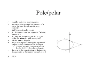
Pole/polar • consider projective geometry again • we may want to compute the tangents of a curve that pass through a point (e.g., visibility) • let C be a conic and x a point • if x lies on the conic, we know that Cx is the tangent at x • if x does not lie on the conic, Cx is a line called the polar of x with respect to C • x is the pole of the polar • the polar of x passes through the 2 points of tangency of the 2 tangents of C through x • if tangent line at y, Cy, contains x, then x^t Cy=0 or (Cx)^t y = 0 so y lies on the polar • the polar is the generalization of the tangent; it degenerates to the tangent when x lies on C • HZ58
Conjugacy • points x and y are conjugate if x^t C y = y^t C x = 0 • if y lies on the polar Cx, then x and y are conjugate • conjugacy is symmetric(!): if y lies on polar of x, then x lies on polar of y • HZ59
Pole/polar for quadrics • quadric Q • polar plane of X = QX • if X lies on Q, QX = tangent plane • if X lies outside Q, QX passes through the points of tangency of the tangent cone through X • HZ73-74
Conic fitting • fitting point data is an important task in shape design • we shall explore in future, but let’s see what projective space has to say first • fitting a conic is equivalent to finding the null space of a matrix • each point (x,y) on a conic imposes a constraint on the conic coefficients • ax^2 + bxy + ... + f = 0 • or, separating the unknowns from the knowns, • (x^2, xy, y^2, x, y, 1) . C = 0, where C = (a,b,c,d,e,f) • 5 points define a 5 x 6 matrix M: MC = 0 • Q: how do you solve for conic C? • A: 1d null space of M defines the coefficients C of the conic • null space computation is also used to find fundamental matrix, epipoles (from F) and camera center (from camera matrix) • HZ31
Projective 3-space • 2D projective geometry was introduced through the duality of lines and points; 3D is motivated through the duality of planes and points; lines are self-dual • plane = 4-vector • point X lies on plane π iff πtX = 0 • projective transformation is represented by a 4x4 nonsingular matrix H: X’ = HX • homographies preserve lines, incidence and order of contact • HZ65-66
3 points plane • consider 3 points Xi that lie on the plane π • build the 3x4 matrix M with ith row = Xit • Mπ = 0 for the plane π • if Xi are in general position, M is rank 3 and its null vector is the plane • if the three points are collinear, M is rank 2 and its 2D null space defines a pencil of planes • i.e., plane = null space of point matrix • the plane can also be expressed through determinants • π = (D234, - D134, D124, - D123)t, where • Dijk = determinant of rows ijk of the 4x3 matrix with ith column = Xi (note that this is transpose of above matrix) • proof: build 4x4 matrix [X,X1,X2,X3], whose determinant = 0 if X is on plane • 3D analogue of line = cross product of two points • equivalently, π = ((X1’ – X3’) x (X2’ – X3’), -X3’t (X1’ x X2’))t where Xi = (Xi’ 1) • 3 planes point is a dual result: null vector of the plane matrix • HZ66-67
Lines • how do you represent a line in 3-space? • line = join of n-1 points or intersection of n-1 planes • shows duality • line has 4dof • can define line by intersection with 2 orthogonal planes (2 parameters per plane) • awkward to represent lines in 3-space since the natural representation by homogeneous 5-vector does not play well with the point and plane’s 4-vectors • see HZ68-70 for representation of lines as null spaces (nice implementation consistency with other results)
Lines as Plücker matrices • the most famous representation of a line is by Plücker • represent the line through points A and B as: • L = AB^t – BA^t • 4x4 skew-symmetric matrix called the Plückermatrix • L is independent of points! • L is rank 2 • L has 4 dof (6 in skew-symm – 1 homogeneous – 1 det 0) • L generalizes 2d line = point x point • valency-2 tensor: if point transforms as X HX, then Plücker matrix transforms as L HLH^t • dual Plücker matrix from two planes: L* = PQ^t – QP^t • point X and line L plane L* X • and L*X = 0 reflects X lying on L • plane X and line L point L X • and LX=0 reflects line L lying in the plane P • HZ70-71
Plücker coordinates and Klein quadric • Plücker coordinates are simply the 6 nonzero elements extracted from the Plücker matrix: {12,13,14,23,42 !,34} • from upper triangle with fifth element reversed • since Plücker matrix is rank 2, det=0 imposes a quadratic constraint on these coordinates: • 12*34 + 13*42 + 14*23 = 0 • dot product of 1st half of L with reversed second half of L • this codimension-1 surface in projective 5-space is called the Klein quadric • two lines L and L’ intersect if and only if L . reversed(L’) = 0 • Klein quadric encodes the fact that a line must intersect itself: L . reversed L = 0 • HZ71-72