Download
1 / 39
390 likes | 556 Views
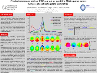
“A User-Friendly Demonstration of Principal Components Analysis as a Data Reduction Method”. R. Michael Haynes, PhD Keith Lamb, MBA Assistant Vice President Associate Vice President Student Life Studies Student Affairs Tarleton State University Midwestern State University.

E N D
“A User-Friendly Demonstration of Principal Components Analysis as a Data Reduction Method” R. Michael Haynes, PhD Keith Lamb, MBA Assistant Vice President Associate Vice President Student Life Studies Student Affairs Tarleton State University Midwestern State University
What is Principal Components Analysis (PCA)? • A member of the general linear model (GLM) where all analyses are correlational • Term often used interchangeably with “factor analysis”, however, there are slight differences • A method of reducing large data sets into more manageable “factors” or “components” • A method of identifying the most useful variables in a dataset • A method of identifying and classifying variables across common themes, or constructs that they represent
Before we get started, aGLOSSARYof terms we’ll be using today: • Bartletts’s Test of Sphericity • Communality coefficients • Construct • Correlation matrix • Cronbach’s alpha coefficient • Effect sizes (variance accounted for) • Eigenvalues • Extraction • Factor or component • Kaiser criterion for retaining factors • Kaiser-Meyer-Olkin Measure of Sampling Adequacy • Latent • Reliability • Rotation • Scree plot • Split-half reliability • Structure coefficients
Desired outcomes fromtoday’s session • Understand the terminology associated with principal components analysis (PCA) • Understand when using PCA is appropriate • Understand how to conduct PCA using SPSS 17.0 • Understand how to interpret a correlation matrix • Understand how to interpret a communality matrix • Understand how to interpret a components matrix and the methods used in determining how many components to retain • Understand how to analyze a component to determine which variables to include and why • Understand the concept of reliability and why it is important in survey research
When is using PCA appropriate? • When your data is interval or ratio level • When you have at least 5 observations per variable and at least 100 observations (ie…20 variables>100 observations) • When trying to reduce the number of variables to be used in another GLM technique (ie….regression, MANOVA, etc...) • When attempting to identify latent constructs that are being measured by observed variables in the absence of a priori theory.
HUERISTIC DATA • Responses to the Developing Purpose Inventory (DPI) collected at a large, metropolitan university between 2004-2006 (IRB approval received) • 45 questions related to Chickering’s developing purpose stage • Responses on 5 interval scale; 1=”always true” to 5=”never true” • Sample size = 998 participants • SUGGESTION: always visually inspect data for missing cases and potential outliers! (APA Task Force on Statistical Inference, 1999). • Multiple ways of dealing with missing data, but that’s for another day!
SPSS 17.0 • Make sure your set-up in “Variable View” is complete to accommodate your data • Names, labels, possible values of the data, and type of measure
SPSS 17.0 • Analyze>Dimension Reduction>Factor
SPSS 17.0 SYNTAXOrange indicates sections specific to your analysis! DATASET ACTIVATE DataSet1. FACTOR /VARIABLES question1 question2 question3 question4 question5 question6 question7 question8 question9 question10 question11 question12 question13 question14 question15 question16 question17 question18 question19 question20 question21 question22 question23 question24 question25 question26 question27 question28 question29 question30 question31 question32 question33 question34 question35 question36 question37 question38 question39 question40 question41 question42 question43 question44 question45 /MISSING LISTWISE /ANALYSIS question1 question2 question3 question4 question5 question6 question7 question8 question9 question10 question11 question12 question13 question14 question15 question16 question17 question18 question19 question20 question21 question22 question23 question24 question25 question26 question27 question28 question29 question30 question31 question32 question33 question34 question35 question36 question37 question38 question39 question40 question41 question42 question43 question44 question45 /PRINT INITIAL CORRELATION SIG KMO EXTRACTION ROTATION FSCORE /FORMAT SORT BLANK(.000) /PLOT EIGEN /CRITERIA MINEIGEN(1) ITERATE(25) /EXTRACTION PC /CRITERIA ITERATE(25) /ROTATION VARIMAX /SAVE AR(ALL) /METHOD=CORRELATION.
OUTPUT COMPONENTS • Correlation Matrix • Pearson R between the individual variables • Variables range from -1.0 to +1.0; strong, modest, weak; positive, negative • Correlations of 1.00 on the diagonal; every variable is “perfectly and positively” correlated with itself! • It is this information that is the basis for PCA! In other words, if you have only a correlation matrix, you can conduct PCA!
OUTPUT COMPONENTS • KMO Measure of Sampling Adequacy and Bartlett’s Test of Sphericity • KMO values closer to 1.0 are better • Kaiser (1970 & 1975; as cited by Meyers, Gamst, & Guarino, 2006) states that a value of .70 is considered adequate. • Bartlett’s Test: you want a statistically significant value • Reject the null hypothesis of a lack of sufficient correlation between the variables.
OUTPUT COMPONENTS • Communality Coefficients • amount of variance in the variable accounted for by the components • higher coefficients =stronger variables • lower coefficients =weaker variables
OUTPUT COMPONENTS • Total Variance Explained Table • Lists the individual components (remember, you have as many components as you have variables) by eigenvalue and variance accounted for • How do we determine how many components to retain?
OUTPUT COMPONENTS • Total Variance Explained Table • Kaiser Criterion (K1 Rule): retain only those components with an eigenvalue of greater than 1; can lead to retaining more components than necessary
OUTPUT COMPONENTS • Total Variance Explained Table • Retain as many factors as will account for a pre-determined amount of variance, say 70%; can lead to retention of components that are variable specific (Stevens, 2002)
Scree Plot Plots eigenvalues on Y axis and component number on X axis Recommendation is to retain all components in the descent before the first one on the line where it levels off (Cattell, 1966; as cited by Stevens, 2002). OUTPUT COMPONENTS
Other Retention Methods • Velicer’s Minimum Average Partial (MAP) test • Seeks to determine what components are common • Does not seek “cut-off” point, but rather to find a more “comprehensive” solution • Components that have high number of highly correlated variables are retained • However, variable based decisions can result in underestimating the number of components to retain (Ledesma & Valero-Mora, 2007)
Other Retention Methods • Horn’s Parallel Analysis (PA) • Compares observed eigenvalues with “simulated” eigenvalues • Retain all components with an eigenvalue greater than the “mean” of the simulated eigenvalues • Considered highly accurate and exempt from extraneous factors (Ledesma & Valero-Mora, 2007)
OUTPUT COMPONENTS • Component Matrix • Column values are structure coefficients, or the correlation between the test question and the synthetic component; REMEMBER: squared structure coefficients inform us of how well the item can reproduce the effect in the component!
Component Matrix Column values are structure coefficients, or the correlation between the test question and the synthetic component; REMEMBER: squared structure coefficients inform us of how well the item can reproduce the effect in the component! Rule of thumb, include all items with structure coefficients with an absolute value of .300 or greater OUTPUT COMPONENTS
Component Matrix For heuristic purposes, we’re retaining the first X components; what variables should we include in the components? Column values are structure coefficients, or the correlation between the test question and the synthetic component; REMEMBER: squared structure coefficients inform us of how well the item can reproduce the effect in the component! Rule of thumb, include all items with structure coefficients with an absolute value of .300 or greater Stevens’ recommends a better way! OUTPUT COMPONENTS
Critical Values for a Correlation Coefficient at α = .01 for a Two-Tailed Test n CV n CV n CV 50 .361 180 .192 400 .129 80 .286 200 .182 600 .105 100 .256 250 .163 800 .091 140 .217 300 .149 1000 .081 (Stevens, 2002, pp. 394) Test the structure coefficient for statistical significance against a two-tailed table based on sample size and a critical value (CV); for our sample size of 998, the CV would be |.081| doubled (two-tailed), or |.162|.
Obtaining Continuous Component Values for Use in Further Analysis • Sum the interval values for the responses of all questions included in the retained component • Obtain mean values for the responses of all questions included in the retained component…hint…you’ll get the same R, R², ß, and structure coefficients as with the sums! • Use SPSS to obtain factor scores for the component • Choose “Scores” button when setting up your PCA • Options include calculating scores based on regression, Bartlett, or AndersonRubin methodologies…be sure and check “Save as Variables” • Factor scores will appear in your data set and can be used as variables in other GLM analyses
RELIABILITY • The extent to which scores on a test are consistent across multiple administrations of the test; the amount of measurement error in the scores yielded by a test (Gall, Gall, & Borg, 2003). • While validity is important in ensuring our tests are really measuring what we intended to measure; “You wouldn’t administer an English literature test to assess math competency, would you?” • Can be measured several ways using SPSS 17.0
RELIABILITY Cronbach’s Alpha Coefficient RELIABILITY /VARIABLES=question1 question2 question3 question4 question5 question6 question7 question8 question9 question10 question11 question12 question13 question14 question15 question16 question17 question18 question19 question20 question21 question22 question23 question24 question25 question26 question27 question28 question29 question30 question31 question32 question33 question34 question35 question36 question37 question38 question39 question40 question41 question42 question43 question44 question45 /SCALE('ALL VARIABLES') ALL /MODEL=ALPHA. Split-Half Coefficient RELIABILITY /VARIABLES=question1 question2 question3 question4 question5 question6 question7 question8 question9 question10 question11 question12 question13 question14 question15 question16 question17 question18 question19 question20 question21 question22 question23 question24 question25 question26 question27 question28 question29 question30 question31 question32 question33 question34 question35 question36 question37 question38 question39 question40 question41 question42 question43 question44 question45 /SCALE('ALL VARIABLES') ALL /MODEL=SPLIT.
RELIABILITY Cronbach’s Alpha Coefficient • Benchmarks for Alpha • .9 & up = very good • .8 to .9 = good • .7 to .8 = acceptable • .7 & below = suspect. “… don’t refer to the test as ‘reliable’, but scores from this administration of the test yielded reliable results”….Kyle Roberts
RELIABILITY Split-Half Coefficient
RELATED LINKS • http://faculty.chass.ncsu.edu/garson/PA765/factor.htm • http://www.uic.edu/classes/epsy/epsy546/Lecture%204%20---%20notes%20on%20PRINCIPAL%20COMPONENTS%20ANALYSIS%20AND%20FACTOR%20ANALYSIS1.pdf • http://www.ats.ucla.edu/stat/Spss/output/factor1.htm • http://www.statsoft.com/textbook/principal-components-factor-analysis/
REFERENCES Gall, M.D., Gall, J.P., & Borg, W.R. (2003). Educational research: An introduction 7th ed.). Boson: Allyn and Bacon. Ledesma, R.D., & Valero-Mora, P. (2007). Determining the number of factors to retain in EFA: an easy-to-use computer program for carrying out parallel analysis. Practical Assessment, Research, & Evaluation,12(2). Meyers, L.S., Gamst, G., & Guarino, A.J. (2006). Applied multivariate research: Design and interpretation. Thousand Oaks, CA: Sage. Stevens, J. P. (2002). Applied multivariate statistics for the social sciences (4th ed.). Mahwaw, NJ: Lawrence Erlbaum Associates. University of California at Los Angeles Academic Technology Services (2009). Annotated SPSS output: Factor analysis. Retrieved January 11, 2010 from http://www.ats.ucla.edu/stat/Spss/output/factor1.htm University of Illinois at Chicago (2009). Principal components analysis and factor analysis. Retrieved January 11, 2010 from http://www.uic.edu/classes/epsy/epsy546/Lecture%204%20---%20notes%20on%20PRINCIPAL%20COMPONENTS%20ANALYSIS%20AND%20FACTOR%20ANALYSIS1.pdf Wilkinson, L. & Task Force on Statistical Inference. (1999). Statistical methods in psychology journals: Guidelines and explanation. American Psychologist, 54, 594-604.