Chapter 4 Vector Graphics
Chapter 4 Vector Graphics. Multimedia Systems. Key Points. Points can be identified by coordinates . Lines and shapes can be described by equations . Approximating abstract shapes on a grid of finite pixels leads to `jaggies'. Anti-aliasing can offset this effect.

Chapter 4 Vector Graphics
E N D
Presentation Transcript
Chapter 4 Vector Graphics Multimedia Systems
Key Points • Points can be identified by coordinates.Lines and shapes can be described by equations. • Approximating abstract shapes on a grid of finite pixels leads to `jaggies'.Anti-aliasing can offset this effect. • Bezier curves are drawn using four control points. • Bezier curves can be made to join together smoothly into paths. • Paths and shapes can be stroked and filled. • Geometrical transformations — translation, scaling, rotation, reflection and shearing — can be applied easily to vector shapes.
Key Points • Three approaches to 3-D modelling are: constructive solid geometry, free-form modelling and procedural modelling. • 3-D rendering models the effect of light and texture, as well as displaying the modelled objects in space. • Ray tracing and radiosity are computationally expensive rendering algorithms that can produce photo-realistic results. • Specialized 3-D applications, such as Bryce and Poser, are easier to use, and may be more efficient, than more general 3-D modelling and rendering systems.
Introduction • Vector Graphics • Compact • Scaleable • Resolution independent • Easy to edit • Attractive for networked multimedia
Introduction • The compactness of vector graphics makes them particular attractive for network multimedia, since the large sizes of the images files lend to excessive download times. • Absence of any standard format for vector graphics prevents it from popularization. • As SVG and SWF standards are adopted, this will change.
Introduction • In vector graphics, images are built up using shapes that can easily be described mathematically. • Vector graphics has been eclipsed (衰退) in recent years by bitmap graphics for 2D images. • Vector graphics is mandatory (強制性) in 3D graphics, since processing voxels is still impractical in modern machines.
Coordinates and Vectors • Image stored as a rectangular array of pixels. • Coordinates (x,y), Fig. 4.1 • Integer • Real coordinate, (2.35, 2.9), Fig. 4.2 • Drawing programs allow to display axes (ruler) along edges of your drawing • Vectors • Approximating a straight line, Fig. 4.4
Coordinates and Vectors • Points A(3,7) B(7,3) O(0,0)
Coordinates and Vectors • Lines
Anti-aliasing • Approximating a straight line • Using intermediate grey values • Brightness is proportional to area of intersection • At expense of fuzziness
Shapes • A simple mathematical representation • Stored compactly and rendered efficiently • Rectangles, squares, ellipses and circles, straight lines, polygons, Bezier curves • Spirals and stars, sometimes • Fills with color, pattern or gradients
Polylines • Rectangles • Ellipses • Curves
Hermite Curves • Hermite parametric cubic curvesC = C(t) = a0 + a1t+ a2t2 + a3 t3 • Four vectors a0 ,a1 ,a2 ,a3 (12 coefficients, 3D) are required to define the curve. • Usually these vectors can be specified by curve’s behavior at end points t=0 and t=1 • Assume endpoints C(0), C(1) tangent vectors, C’(0), C’(1) are given, then a0 = C(0) a1 + a2 + a3 = C(1) a1 = C’(0) a1 +2 a2 + 3 a3 = C’(1)
T1 T0 Hermite Curves • a0 = C(0)a1 = C’(0)a2 = 3( C(1) - C(0)) - 2C’(0) - C’(1)a3 = 2 ( C(0) - C(1)) + C’(0) + C’(1) • C(t) = (1-3t2 + 2t3) C(0) + (3t2 -2t3) C(1) + (t - 2t2 + t3) C’(0) + (-t2 + t3) C’(1)) • C(t) = [1 t t2 t3] 1 0 0 0 C (0) 0 0 1 0 C (1) -3 3 3 -2 C’(0) 2 -2 1 1 C’(1)
Bezier Curves • Given four control points b0, b1, b2 , b3, then the corresponding Bezier curve is given byC(t) = (1-t)3b0 + 3t(1-t)2b1 + 3t2(1-t)b2 + t3b3C’(t) = -3(1-t)2b0 + 3(1-4t+3t2)b1 + 3(2t-3t2)b2 + 3t2b3 • C(0)=b0C(1)=b3C’(0)=3(b1-b0)C’(1)=3(b3-b2)
Bezier Curves • C(t) = [1 t t2 t3] 1 0 0 0 b0 -3 3 0 0 b1 3 -6 3 0 b2 -1 3 -3 1 b3 b1 b2 b3 b0
Bezier Curves • Four control points • Two endpoints, two direction points • Length of lines from each endpoint to its direction point representing the speed with which the curve sets off towards the direction point • Fig. 4.8, 4.9
Bezier Curves • Constructing a Bezier curve • Fig. 4.10-13 • Finding mid-points of lines
Bezier Curves • Figs. 4.14-18 • Same control points but in different orders
Bezier Curves b11 b1 b2 b12 b02 b03 b01 b21 b0 b3
Bezier Cubic Curves • x(t) = ax t3 +bxt2 + cxt + x1y(t) = ay t3 +byt2 + cyt + y1 • p1= (x1, y1) • p2=(x1 + cx/3, y1 + cy/3) • p3=(x2 + (cx +bx )/3, y2 + (cy +by )/3) • p4=(x1 + cx +bx +ax, y1 + cy +by +ay)
Smooth Joins between Curves • Fig. 20 • Length of direction linesis the same on each side • Smoothness of joins when control points line up and direction lines are the same length • Corner point • Direction lines of adjacent segments ate not lines up, Fig. 4.21
Changing a smooth curve to a corner and vice versa convert-anchor-point tool
Paths • Joined curves and lines • Open path • Closed path
Each line or curve is called a segment of the path • Anchor points: where segments join • Pencil tool: freehand • Bezier curve segments and straight lines are being created to approximate the path your cursors follows • A higher tolerance leads to a more efficient path with fewer anchor points which may smooth out of the smaller movements you made with pencil tool
Stroke and Fill • Apply stroke to path • Drawing program have characteristics such as weight and color, which determine their appearance. • Weight= width of stroke • Dashed effects • Length of dashes • Gaps between them
Line Caps & Joins • Line cap • Butt cap • Round cap • Projecting cap • Line Joins • Miter • Rounded • Bevel
Fill • Most drawing programs also allow to fill an open path • Close the path with straight line between its endpoints • Flat color, pattern or gradients • Gradient: linear, radial • Texture
Fill • Pattern • Tiles: a small piece of artwork • Use pattern to stroke paths, a textured outline • Arrange perpendicular to path, not horizontally • Include special corner tiles • If you want to fill a path, you need to know which areas are inside it. (Fig. 4.27) • Non-zero winding number rule • Draw a line from the point in any direction • Every time the path crosses it from left to right, add one to winding number; every time the path crosses from right to left, subtract one from winding number • If winding number is zero, the point is outside the path, otherwise it is inside. • Depends on the path’s having a direction
Transformations and Filters • Transformations • Translations: linear movement • Scaling, rotation about a point • Reflective about a line • Shearing: a distortion of angles of axes of an objects
Filters • Free manipulation of control points • Roughening • moves anchor points in a jagged array from the original object, creating a rough edge on the object
Scribbling filter • randomly distorts objects by moving anchor points away from the original object
Rounding • converts the corner points of an object to smooth curves • Filter > Stylize > Round Corners • Only relatively few points need to be re-computed
3-D Graphics • Axes in 3D: Fig. 4.35 • Rotations in 3D: Fig. 4.36
3-D Graphics • Right-handed coordinate system, Fig. 4.37 • 2D: define shapes by paths3D: define objects by surfaces • Hierarchical modeling • A bicycle consists of a frame, two wheels, …
Rendering • In 3D, we have a mathematical model of objects in space, but we need a flat picture. • Viewpoint • Position of camera • Scaling with distance • Lighting: position, intensity, type • Interaction of light: underwater, smoke-filled room • Texture • Physical impossibilities: negative spotlights, absorbing unwanted light
3D Models • Constructive solid geometry • A few primitive geometric solids such as cube, cylinder, sphere and pyramid as elements from which to construct more complex objects • Operators: union, intersection, and difference, Figs. 38-40 • Physical impossibility
Free Form Modeling • Mesh of polygons • A certain regular structure or symmetry from 2D shapes • Treat a 2D shape as cross section and define a volume by sweeping the cross section along a path • Extrusion • To produce more elaborate objects • Curved path can be used • Size of cross section can be altered • Lathing
Procedural Modeling • Models described by equations • Fractals, Fig. 4.42 • Coastlines • Mountains • Edges of cloudy • Fig. 4.43, snowflake • Fractal mountainside, Fig. 4.44
Procedural Modeling • 3D Fractals • Fig. 4.45 • Fractal terrain, Fig. 4.46
Procedural Modeling • Metaballs • Model soft objects • Fig. 4.47 • Complex objects can be built by sticking metaballs together • Particle systems • Features made out of many particles • Rains, fountains, fireworks, grass
Metaballs • Metaballs are also included and make a great addition to helping create base models for further editing.A Metaball can be used in either a positive or negative way in trueSpace 5.
Lightwave • Particle explosion • Particle Storm 2.0
Rendering • Wire frame, Fig. 4.48 • Hidden surface removal • Surface properties • Color and reflectivity • Lights • Shading • A color for each polygon • Interpolate color • Gouraud shading • Phong shading: specular reflection
Ray tracing • Tracing the path of a ray of light back from each pixel , Plate 8 • Photo-realistic graphics • High-performance workstations • Radiosity • Interactions between objects • Model complex reflections that occur between surfaces that are close together