Download
1 / 49
490 likes | 602 Views
This document outlines the revisions and analyses of target atmospheres used for space-based Doppler Wind Lidar (DWL) concepts, presented during the WG meeting by G. D. Emmitt and S. A. Wood. It reviews the historical context, comparison with ESA's data, and methodologies utilizing FASCODE/MODTRAN models. The study includes discussions on wavelength scaling, depolarization effects, solar background impacts, and air mass classifications. The results aim to enhance OSSEs (Observing System Simulation Experiments) for more effective climate monitoring using advanced remote sensing techniques.

E N D
Revisiting Target Atmospheres for Space-based DWL Concept Comparisons G. D. Emmitt and S. A. Wood Simpson Weather Associates October 16 – 18, 2012 WG meeting in Boulder, CO
Outline • Background on Target Atmospheres • Comparison with ESA’s data base • Comparison with FASCODE/MODTRAN • Wavelength scaling • Role in OSSEs • Areas for enhancement • Depolarization • Solar background • Multiple air-mass classifications
Background on Target Atmospheres • Developed in 1997 for use in trade studies and comparisons of DWLs operating at differing wavelengths. • Co-authored by Emmitt, Spinhirne, Menzies, Winker and Bowdle • Published on www.swa.com • Underwent several revisions as new data with 2 um, 1.06 um and .532 um observations became available.
TARGET ATMOSPHERES for use in DWL CONCEPT STUDIES Submitted to the New Millennium Program by An Ad Hoc Committee: G.D. Emmitt, Lead Simpson Weather Associates, Charlottesville, VA J. Spinhirne NASA/GSFC, Greenbelt, MD R. Menzies NASA/JPL, Pasadena, CA D. Winker NASA/LaRC, Hampton, VA D. Bowdle NASA/GHCC, Huntsville, AL March 28, 1997 (1st draft) May 2, 1997 (2nd draft) July 23, 1997 (3rd draft) February 2, 1998 (4th draft with edits by gde) August 10, 2001(Edits by gde) The following material was put together in its original form at the request of the participants of the March 1997 NMP Lidar Workshop held in Washington, D.C. Subsequently, revisions have been made, in part, in response to request for more complete representation of the attenuation coefficients.
Current Target Atmospheres • The basic backscatter profiles from surface to 25 km were scaled from .532 GLOBE observations. Molecular backscatter, total scatter, attenuation were derived using FASCODE. • Angstrom exponents used: λ-2.5 above 3 km and λ-1.5 at and below 3 km. • Added some cloud and wind turbulence for use in instrument trade studies.
DESIGN ATMOSPHERES for use in GTWS CONCEPT STUDIES** provided by the Science Definition Team for the NASA/NOAA Global Tropospheric Wind Sounder September 22, 2001 Purpose Having a common scattering target with internally consistent backscatter wavelength dependence enables meaningful "equal resource/equal target“ comparisons of GTWS concepts that employ Doppler lidars. While the Science Definition Team (SDT) realizes that aerosol backscatter from the atmosphere will vary over several orders of magnitude, will vary over altitude, latitude and season and will also vary over space/time scales that are not readily modeled, the GLOBE , SABLE/GABLE backscatter surveys, and the AFGL MODTRAN aerosol data bases provide a nearly consistent picture of backscatter climatology.
Comparison with ESA’s Data Base Establishment of a backscatter coefficient and atmospheric database Work performed with funding from ESA to DERA J. M. Vaughan, N. J. Geddes, Pierre H. Flamant and C. Flesia June 1998
Comparison with FASCODE • Many engineers use MODTRAN/FASCODE in assessing performance of DWL concepts. • With a focus on the aerosol returns from the lower troposphere, we find that FASCODE/MODTRAN provides backscatter values ~ 10 – 30 times higher than those in our Target Atmospheres’ “background mode”. Comparisons at 1 km and .355um
Scaling Issues • Scaling expressed using an Angstrom Exponent or a Color Ratio. • Much of ESA’s backscatter database derived from 10.6 um observations in SABLE and GABLE in the Atlantic in 1988-1990 using a simple expression for the Angstrom Exponent. • NMP’s Target Atmospheres derived from 1.06 um and .532um observations made in GLOBE 1990 over the Pacific using two differing Angstrom Exponents. • The following few slides are based upon modeling done with NASA/ROSES funding for the analyses of CALIPSO data. Modeling done by Kirk Fuller (UAH)
.355um .532 1.06 2.06 For reference: using λ-2.5 ; β14 = 81.1 using λ-1.5 ;β14=13.9 Dr. Kirk A. Fuller July 8, 2010 University of Alabama in Huntsville
bi/ bjfor Fine Dust Dr. Kirk A. Fuller July 8, 2010 University of Alabama in Huntsville
bi/ bjfor Coarse Dust Dr. Kirk A. Fuller July 8, 2010 University of Alabama in Huntsville
bi/ bjfor Bimodal Dust Dr. Kirk A. Fuller July 8, 2010 University of Alabama in Huntsville
bi/ bjfor Fine Polluted Dust Dr. Kirk A. Fuller July 8, 2010 University of Alabama in Huntsville
bi/ bjfor Coarse Polluted Dust Dr. Kirk A. Fuller July 8, 2010 University of Alabama in Huntsville
bi/ bjfor Bimodal Polluted Dust Dr. Kirk A. Fuller July 8, 2010 University of Alabama in Huntsville
bi/ bjfor Fine Clean Marine Dr. Kirk A. Fuller July 8, 2010 University of Alabama in Huntsville
bi/ bjfor Coarse Clean Marine Dr. Kirk A. Fuller July 8, 2010 University of Alabama in Huntsville
bi/ bjfor Bimodal Clean Marine Dr. Kirk A. Fuller July 8, 2010 University of Alabama in Huntsville
bi/ bjfor Fine Clean Continental Dr. Kirk A. Fuller July 8, 2010 University of Alabama in Huntsville
bi/ bjfor Coarse Clean Continental Dr. Kirk A. Fuller July 8, 2010 University of Alabama in Huntsville
bi/ bjfor Bimodal Clean Continental Dr. Kirk A. Fuller July 8, 2010 University of Alabama in Huntsville
bi/ bjfor Fine Polluted Continental Dr. Kirk A. Fuller July 8, 2010 University of Alabama in Huntsville
bi/ bjfor Coarse Polluted Continental Dr. Kirk A. Fuller July 8, 2010 University of Alabama in Huntsville
bi/ bjfor Bimodal Polluted Continental Dr. Kirk A. Fuller July 8, 2010 University of Alabama in Huntsville
bi/ bjfor Fine Dry Smoke Dr. Kirk A. Fuller July 8, 2010 University of Alabama in Huntsville
bi/ bjfor Coarse Dry Smoke Dr. Kirk A. Fuller July 8, 2010 University of Alabama in Huntsville
bi/ bjfor Bimodal Dry Smoke Dr. Kirk A. Fuller July 8, 2010 University of Alabama in Huntsville
Three primary classes of aerosols General derivations of backscatter at 2.01 um from observations at .355um Example: Beta 2.01 = (2.01/.355)^-2.18 *Beta .355= .022 *Beta .355
Issues for OSSEs • Strategy is to keep the optical property modeling as simple as possible and consistent with the information provided by the Nature Run. • Currently we add sub-grid scale turbulence based upon model wind variability on its grid scale. • We derive cloud optical properties (optical depth) from model provided cloud and water phase information. • We run the experiments with three options for aerosol distribution: • Entire globe in background • Entire globe in enhanced mode • Backscatter (background through enhanced) organized by model RH fields
Areas for Enhancement • Employ a first order, source anchored set of air-mass types with differing backscatter (this was done in some of the first DWL simulations for OSSEs in the early 1990’s) • Add depolarization effects by clouds (especially thin cirrus) • Add solar background in a more advanced fashion (groundand clouds). Not just day/night adjustments to SNR.
Discussion • Given the constraints associated with OSSEs, how should we upgrade the Target Atmospheres, if at all? • What process should we use to vet changes?