Download
1 / 46
480 likes | 635 Views
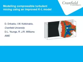
Modelling compressible turbulent mixing using an improved K-L model. D. Drikakis, I.W. Kokkinakis, Cranfield University D.L. Youngs, R .J.R. Williams AWE. Outline. Modified K-L model Two-fluid model Implicit Large Eddy Simulations Eulerian finite volume

E N D
Modelling compressible turbulent mixing using an improved K-L model D. Drikakis, I.W. Kokkinakis, Cranfield University D.L. Youngs, R .J.R. Williams AWE
Outline • Modified K-L model • Two-fluid model • Implicit Large Eddy Simulations • Eulerian finite volume • Lagrange-Remap • Assessment of turbulence models vs. ILES for compressible turbulent mixing • 1D Rayleigh-Taylor • Double Planar Richtmyer-Meshkov • Inverse Chevron Richtmyer-Meshkov • Conclusions and future work
Motivation • Direct 3D simulation of the turbulent mixing zone in real problems is impractical. • Alternative: Engineering turbulence models to represent the average behaviour of the turbulent mixing zone. • Aim: To develop and asses a range of engineering turbulence models for compressible turbulent mixing
K-L model Favre-averaged Euler multi-component equations: • Fully-Conservative form (4-equation) • Assume turbulent mixing >> molecular diffusion (viscous effects) Continuity: Additional Terms Require Modelling Momentum: Total Energy: Mass-Fraction:
K-L model (cont.) Two-equation turbulent length-scale-based model (K-L): • Originally developed by Dimonte & Tipton (PoF, 2006); • RANS-based linear eddy viscosity model; • Achieves self-similar growth rates for initial linear instability growth. Turbulent kinetic energy: Turbulent length scale:
K-L model (cont.) Additional closure terms: Boussinesq eddy viscosity assumption Turbulent viscosity Turbulent velocity Turbulent dissipation rate Acceleration of fluids interface due to pressure gradient Turbulent energy (K) production Mean flow timescale RM-like RT-like Turbulent timescale
Turbulent production source term limiter (SK) At late time, the model over-predicts the production of the total kinetic energy: • a posteriori analysis indicates that a threshold in the production of K is reached when the eddy size L exceeds a certain value of the mixing width (at the first interface) • and the K source production term becomes:
Limiting the eddy viscosity • Limiting the turbulent viscosity affects the terms: Turbulent Shear Stress Turbulent Diffusion • Rescale turbulent viscosity (μT) using a limiter, SF : Tangential velocity to the cell face Local speed of sound
Atwood number calculation The original K-L model calculates the local cell Atwood number (ALi) based on the van Leer’s Monotonicity principle:
Modified K-L, Atwood Number • Uses the average values obtained during the reconstruction phase of the inviscid fluxes to estimate the: • local Atwood number; • gradients in turbulence model closure and source terms. • Weighted contribution of ASSi and A0i to obtain ALi
Modified K-L, Atwood Number Reconstructed values (F)
Modified K-L: Enthalpy diffusion Replaced turbulent diffusion of internal energy (qe) with enthalpy (qh), based on suggested physical diffusion mechanism (A.Cook, PoF, 2009) where:
Modified K-L Summary of modifications introduced to the original K-L (Dimonte & Tipton): • Changed the internal energy turbulent diffusion flux to the enthalpy one • Make use of reconstruction values at the cell face to calculate the: • local Atwood number; • turbulence model closure and source terms; • turbulent viscosity for diffusion; • The local Atwood number is calculated using weighted contributions • Introduced an isotropic turbulent diffusion correction for 2D simulations • Reduce late time turbulent kinetic energy production
Young’s Two-Fluid Model • Mass transport: • Momentum transport: • Internal energy: • Volume fraction:
Two-Fluid Model (cont.) • An equation for K is used which is similar to that in the K-L model but with a different source term: • The equation for L includes a source term involving fluid velocity differences and is different to that used in the K-L model: • Turbulent viscosity is given by: where ℓt is proportional to L, turbulent diffusion coefficients are proportional to ℓt K1/2.
Two-Fluid Model (cont.) is the fraction by mass of initial fluid p in phase r is the rate of transfer of volume from phase r to phase s;determines how rapidly the initial fluids mixat a molecular level. is the rate of transfer of momentum from phase s to phase r accounting for drag, added mass and mass exchange. • Model coefficients are chosen to give an appropriate value of α for RT mixing (typically 0.05 to 0.06); • The volume transfer rate ΔVrs is chosen to give the corresponding value of the global mixing parameter for self-similar RT mixing; • The ratio ℓt /L is chosen so that a fraction of about 0.3 to 0.4 of mixing for self-similar RT is due to turbulent diffusion.
Implicit Large Eddy Simulation CNS3D code • CNS3D code: Finite volume approach in conjunction with the HLLC Riemann solver • Several high-resolution and high-order schemes • 2nd-order modified MUSCL (Drikakis et al., 1998, 2004) • 5th-order MUSCL (Kim & Kim) and WENO (Shu et al.) • 9th-order WENO for ILES (Mosedale & Drikakis, 2007) • Specially designed schemes incorporating low Mach corrections (Thornber et al., JCP, 2008) • 5-equation quasi-conservative multi-component model (Allaire et al., JCP, 2007) • 3rd-order Runge-Kutta in time
Lagrange-Remap AWE TURMOIL code • TURMOIL code: Lagrange-Remap method (David Youngs) • 3rd-order spatial remapping; • 2nd-order in time; • Mass fraction mixture model. • For the semi-Lagrangian scheme • Lagrangian phase: • Quadratic artificial viscosity; • Negligible dissipation in the absence of shocks. • Remap phase: • 3rd-order monotonic method; • Mass and momentum conserved. The kinetic energy is dissipated only in regions of non-smooth flow.
Turbulent Mixing Instabilities Three cases are investigated: • 1D Planar RT (1D-RT); • 1D Double Planar RM (1D-RM); • 2D Inverse Chevron (2D-IC); • Shear at the inclined interface subsequently results in formation of Kelvin-Helmholtz (KH) instabilities.
Validation The model results are compared against high-resolution ILES: • Profiles of volume fraction (VF); • Profiles of turbulent kinetic energy (K); • Integral quantities such as the Total MIX and Total Turbulent Kinetic Energy (Total TKE) are employed: • For comparison with 2D RANS simulations, the 3D ILES results are Favre-averaged to a 2D plane in the homogeneous spanwise direction, and a surface integral is applied instead; • The results need to be multiplied with a spanwise length (Lz) for consistency with the 3D quantities.
FLUID PROPERTIES G=1.105cm2/s ρH=20gr/cm3 ρL=1gr/cm3 Pint=1000dyn/cm2 γH≠ γL Atwood Number ≈ 0.90 Rayleigh-Taylor
Effect of Enthalpy Diffusion Comparison of static Temperature profiles against Two-Fluid model (TF):
Effect of Enthalpy Diffusion Comparison of VF and K profiles against Two-Fluid model (TF) and high-resolution ILES (Youngs 2013):
Effect of Enthalpy Diffusion The modified model gives correct self-similar growth rates of mixing width (W) and maximum turbulent kinetic energy (KMAX):
FLUID PROPERTIES P=1bar ρsf6=6.34kg/m3 ρair=1.184kg/m3 U*air=131.196m/s P*air=1.675bar ρ*air=1.7047kg/m3 Atwood Number 0.67 Richtmyer-Meshkov
VF-profiles t=1.90ms t=2.22ms
VF-profiles (cont.) t=2.70ms t=3.82ms
TKE-profiles t=1.90ms t=2.22ms
TKE-profiles (cont.) t=2.70ms t=3.82ms
Inverse Chevron FLUID PROPERTIES Favre-averaged 3D initial condition to 2D plane for mean flow quantities. ρsf6=6.34kg/m3 ρair=1.184kg/m3, ρ*air=1.7264kg/m3 P*air=1.706bar , P=1bar Shock Mach Number=1.26 Atwood Number 0.67
1280x640x320 resolution (Hahn et. al., PoF, 2011) 1.9ms 2.7ms 3.3ms 3D High-Resolution ILES EXP K1 KMIN2
K-L model applied to IC • 2D K-L turbulence model on 320x160 cells in x and y-directions; • Complete on standard multi-core desktop PC within an hour; • Assumes mean flow is zero in z-direction (only fluctuations). Challenges: • Strong anisotropic turbulent effects; • Late time turbulent energy production; • De-mixing.
Evolution of VF (ILES) t=0.5ms t=1.3ms t=1.9ms t=3.3ms t=2.2ms t=2.7ms
VF contours at t=2.7ms KL ILES TF KL modified
VF contours at t=3.3ms KL ILES TF KL modified
Evolution of TKE (ILES) t=0.5ms t=1.3ms t=1.9ms t=3.3ms t=2.2ms t=2.7ms
TKE contours at t=2.7ms KL ILES TF KL modified
TKE contours at t=3.3ms KL ILES TF KL modified
Conclusions • Both models achieve self-similarity. • The correct treatment of the enthalpy flux is required in the K-L model in order to improve the model results. • Modifications in the calculation of the local Atwood number and limiting the turbulent viscosity and production of TKE significantly improve the K-L results. • The TF model overall predicts more accurately the K/Kmax profile. • The TF model gives more accurate results than the KL model at late times, where anisotropy and de-mixing dominates. • A key advantage of the TF model is its capability of representing the degree of molecular mixing in a direct way, by transferring mass between the two phases.