Download
1 / 51
510 likes | 710 Views
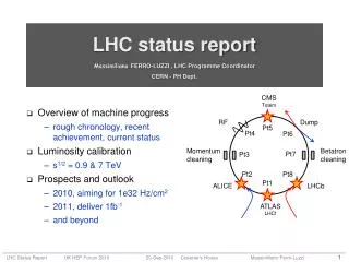
CMS Totem. LHC status report Massimiliano FERRO-LUZZI , LHC Programme Coordinator CERN - PH Dept. RF. Dump. Pt5. Pt4. Pt6. Momentum cleaning. Betatron cleaning. Pt7. Pt3. Overview of machine progress rough chronology, recent achievement, current status Luminosity calibration

E N D
CMS Totem LHC status reportMassimilianoFERRO-LUZZI , LHC Programme CoordinatorCERN - PH Dept. RF Dump Pt5 Pt4 Pt6 Momentum cleaning Betatron cleaning Pt7 Pt3 Overview of machine progress rough chronology, recent achievement, current status Luminosity calibration s1/2 = 0.9 & 7 TeV Prospects and outlook 2010, aiming for 1e32 Hz/cm2 2011, deliver 1fb-1 and beyond Pt2 Pt8 Pt1 ALICE LHCb ATLAS LHCf
Rough chronology Oct 2008 – Oct 2009: recovered from s34 incident 20 Nov 2009: Resuming (circulating) beam commissioning 6 Dec 2009: First physics collisions at 450 GeV/beam 13-14 Dec 2009: Ramps and collisions to 1.18 TeV/beam Mid Dec 2009 – End Feb 2010 --- Technical stop 27 Feb 2010: Started LHC (first beams 2010), commissioning 20 Mar 2010: First ramps to 3.5 TeV 30 Mar 2010: First physics collisions at 3.5TeV/beam 23 Apr 2010: First run with squeezed optics (* = 2m) mid Jun 2010: Go to *=3.5 m, push bunch&beam intensity 25 Jun 2010: First physics with nominal bunches (*=3.5 m) 19 Aug 2010: Exceeded 2 MJ/beam in physics (2.7 MJ). mid Sep 2010: Bunch trains, crossing angle end 2010: Reach ~1e32 Hz/cm2
Integrated lumi (delivered, in STABLE BEAMS) Plots at http://cern.ch/lpc setting up nominal bunches 2m / LHCf** / LHCf** ** LHCf: out since 20 july 2010 ** LHCf: out since fill 1250 Goal end 2011: 1 fb-1 Also: ~360 ub-1 at 450GeV/beam and ~1 ub-1 data with 1.18 TeV/beam
Peak luminosity (delivered, in STABLE BEAMS) / LHCf** / LHCf** ** LHCf: out since 20 july 2010 ** LHCf: out since fill 1250 Goal end 2010: ~ 1e32 Hz/cm2 = 100 Hz/ub During 2011: exceed 2e32 Hz/cm2 = 200 Hz/ub
2008 sector 3-4 incident remember this ?
LHC stored energy s34 incident • Despite modest luminosity (1e31 Hz/cm2) we are at 2.7 MJ • Nominal LHC • A factor 2 in magnetic field • A factor 7 in beam energy • A factor 200 in stored energy! 360 MJ 2808x1.1 1011p LHC 2010-2011 target 4x72x1.1 1011p Done to date
Increasing stored energy in the LHC beams Reach approx 20 MJ by end of 2010, approx 30 MJ by end of 2011 linear Y scale log Y scale apr may junjulaug apr may junjulaug 3 MJ
Beam cleaning, regular monitoring • so far , so good! (very stable, no readjustments over ~2 months) • not a single quench os SC magnet with circulating beam Beam 1 vertical losses BLM dump levels IR3 IR7
A typical recent fill (end of August) as imaged by vtx detectors • lumi life time ~25 h • due to both beam current decrease and to transverse emittance blow-up • here about 20% in current and 20% in emittance per plane over 13h ATLAS CMS LHCb “L” “L / (N1 N2)” “L dt”
Overview Thu 29.07.2010 22:00 to Tue 18.08.2010 10:00 Given a total time T, a delivered lumiL and a peak lumiL, define an “overall factor” for quick estimations (Hűbner): L H = ––––– T L At LEP & Tevatron, H ~0.2-0.25 in their late years…
From Thu 29.07.2010 22:00 to Tue 18.08.2010 10:00 total time T : 468h time in stable beams : 153.7 h delivered lumiL : 1.2 pb-1 typical peak lumi L : 2.5 to 4 Hz/ub All fills with 25 bunches, 3.5m, 3.5 TeV: FillNr 1251, Thu 29.07.2010 23:28 => Fri 30.07.2010 07:25 ~8.0h FillNr 1253, Fri 30.07.2010 23:11 => Sat 31.07.2010 12:20 ~13.1h FillNr 1256, Sun 01.08.2010 03:50 => Sun 01.08.2010 04:49 ~1.0h FillNr 1257, Sun 01.08.2010 22:00 => Mon 02.08.2010 12:35 ~14.5h FillNr 1258, Tue 03.08.2010 00:22 => Tue 03.08.2010 07:39 ~7.3h FillNr 1260, Wed 04.08.2010 04:31 => Wed 04.08.2010 06:38 ~2.1h FillNr 1262, Wed 04.08.2010 17:40 => Thu 05.08.2010 11:19 ~17.65h FillNr 1263, Fri 06.08.2010 03:52 => Fri 06.08.2010 19:08 ~15.25h FillNr 1264, Sat 07.08.2010 01:42 => Sat 07.08.2010 02:14 ~0.5h FillNr 1266, Sat 07.08.2010 23:12 => Sun 08.08.2010 01:10 ~2.0h FillNr 1267, Sun 08.08.2010 05:18 => Sun 08.08.2010 18:52 ~13.5h FillNr 1268, Mon 09.08.2010 01:29 => Mon 09.08.2010 04:02 ~2.5h FillNr 1271, Tue 10.08.2010 07:24 => Tue 10.08.2010 12:22 ~5.0h FillNr 1283, Fri 13.08.2010 23:06 => Sat 14.08.2010 12:04 ~13.0h FillNr 1284, Sat 14.08.2010 15:44 => Sat 14.08.2010 19:13 ~3.5h FillNr 1285, Sun 15.08.2010 00:39 => Sun 15.08.2010 13:02 ~12.4h FillNr 1287, Sun 15.08.2010 23:01 => Mon 16.08.2010 09:24 ~10.4h FillNr 1293, Tue 18.08.2010 09:12 => Tue 18.08.2010 21:13 ~12.0h L H = ––––– = 0.18 to 0.28 T L (caveat: this is a 3-week period with no technical stop) fraction time in stable beams: 32.8%
Why luminosity determination is important Rate = Luminosity x Cross section • Allows to determine cross section of interaction processes on an absolute scale • At the LHC: Heavy flavour production, couplings of new particles, total (inelastic, elastic) cross section, … ( => what precision should we aim for ? ) • Allows to quantify the performance of the collider • Important to verify experimental conditions, to understand quantitatively beam-beam effects, …
Luminosity measurements • First absolute normalisation of luminosity and cross section were performed at the LHC (450 GeV / beam and 3.5 TeV / beam) • Two direct methods were used: • van der Meer method: measure reaction rate vs beam transverse separation • beam-gas imaging method: reconstruct vertices of interactions with residual gas => get the beam profiles • Results accuracy dominated by beam current normalisation uncertainty (~10%, being worked on) • Potentially, could hope to aim for total uncertainty ~5% (future measurements) • will first have to work hard on the beam current normalisation • then on other smaller systematic uncertainties revolution freq bunch populations crossing angle beam overlap new!
Chronology 2009 • All experiments started off with a normalisation based on a generator model including detector simulation => uncertainties at the level of 20% for 450 GeV • LHCb performed first direct luminosity normalisation at 450 GeV using the beam-gas imaging method (see later) 2010 • At 3.5 TeV, started off again with a normalisation based on a generator model including detector simulation • Then, April-May, performed first direct luminosity measurement at each IP with van der Meer scans (+continuous beam-gas imaging normalisation, LHCb)
Van der Meer’s trick Consider single circulating & colliding bunch pair with zero crossing angle R = L = f N1 N2 1(x,y) 2(x,y) dx dy With transverse displacements x , y of one beam w.r.t. the other: R (x , y) = L(x , y) = f N1 N2 1(x-x , y-y) 2(x,y) dx dy R (x , y) dx dy = f N1 N2 1(x-x , y-y) 2(x,y) dx dy dx dy = f N1 N2 2(x,y) [ 1(x-x , y-y) dx dy] dx dy = f N1 N2 2(x,y) dx dy = f N1 N2 x z =1 =1
Assumptions… • Beams do not change when they are moved across each other • correct for (or neglect) beam-beam effects • correct for (or neglect) slow emittance growth • correct for (or neglect) slow bunch current decay • Scan range sufficiently large to cover the distributions • negligible tails • Relation between transverse displacement parameters (magnet currents) and the actual displacement is known on absolute scale • calibrate the absolute displacement scale with vertex detectors
LHCb scans (fill 1059) • 4 scans • L0CaloRate corrected for small pile-up effect • Checked rate at “working point” R(x0 , y0), red points, throughout the scans (~1h) • correct for small decay (~30 h life time)
Van der Meer scans • Scans done at all IPs • 2xIP1 • 2xIP5 • 1xIP8 • 1xIP2 • Profit from modest bunch charge (small beam-beam effects) • First attempts, give ~10% uncertainty on absolute luminosity determination • Uncertainty dominated by knowledge of individual bunch populations
Beam-gas imaging method residual gas Again, luminosity L = f N1 N2 2c cos2(/2) 1(r,t) 2(r,t) d3r dt • Beam interacts with residual gas around the interaction region • Reconstruct beam-gas interaction vertices => sample transverse beam profile measure individually the 1 and 2 and rebuild the overlap (measure also and hourglass effect and and and…) • Strength with respect to van der Meer method: (a) non disruptive, do not affect the beams! (b) can run fully parasitically during physics running time => potentially smaller systematics uncertainties • Requires: • vtx detector resolution smaller (or at least comparable) to the beam sizes • residual pressure & acceptance must be adapted to this method
The LHCb VELO as a beam imaging device • At 450 GeV the VELO is not fully closed around the beam (for safety reasons) • Still, can reconstruct the beams!
Example, 450 GeV beam imaging (2009) Angle from dipole spectrometer bump Crossing type: beam1-beam2 beam1-empty empty-beam2 And the VELO was not even closed around the beams…
LHCb beam-gas imaging and VdM results at 3.5 TeV • Agreement between two methods (vdm and beam-gas) • Thin error bars include beam current normalisation uncertainty • Thick error bars: without beam current normalisation uncertainty P = cross section of event with 2 or more RZVelo tracks
Outlook what next ? end of 2010 2011 and long term
Luminosity parameters f kb N2 L = ––––––– = 1e31 Hz/cm2(as obtained) 4 * T The only parameter which is still very far away from a “realistic 2011 target” is the number of bunches using T =3.3 um , N=1e11 , kb=35 , *=3.5m or desired
Highest priority for Autumn 2010 Get a few hundred nominal bunches stably colliding in the LHC • Reduced bunch spacing • opted for 150ns spacing to start with • will allow up to ~400 bunches • next year, move to 50 ns or 75 ns • Requires crossing angle in all IRs • avoid parasitic collisions away from IP • still get many long-range collisions between bunches (up to 18 long-range + 3 head-on collisions for some bunches) • beam-beam effects ? • minimum crossing angle ? How easy will it be ? 45 m “long range” collision
Fast local loss evts: occurrence scaling with intensity ? • 7 such events have provoked non-programmed dumps (prematurely interrupted a fill) • Time scale of losses ~1-2 ms • These events have occurred in the whole machine (no obvious preference for an area) No proven explanation of these events (yet) A hypothesis: “dust particles” or “shards” traversing the beam Very preliminary plot by Tobias Baer & JorgWenninger Under investigation
Quench test , 18-19 sep 2010 • Beam1 bump beam inward at 14R2.B1, by up to 24mm • One bunch of ~8e9p , “inject and dump” mode • BLM thresolds raised a factor 3 above calculated quench level • no quench…
Beam-beam effects • Scanning crossing angle at injection (450 GeV), online observations
Commissioning bunch trains All done by now
Speeding up the turn-around time • going from 2A/s to 10A/s ramp rates
Great optics Excellent reproducibility
Many more nice results from recent hard work… Unfortunately, no time to show them all… • Dump protection: revalidating with the newly defined machine • RF: preparing for hundreds of bunches • all cavities are on at reduced voltage, adjusted longitudinal blow-up, bunch length reduced from 1.4ns to 1.2ns (and later to the nominal 1ns?) • Beam instrumentation, continuous improvements • Aperture studies • etc. A lot of work done by our machine colleagues in the past 2 weeks which sets the basis for moving from ~50 bunches (2.7 MJ) all the way to 400 bunches (22 MJ) before end of November.
150ns filling schemes: a possible evolution actual PS trains IP2 bunches (=collisions)
LHC schedule, 2010 Heavy Ion run: • magnetically as for pp, except crossing scheme • up to at least 62 bunches, 8e24 Hz/cm2, or more ? 48 96 192 240 336 144 288 384
2011 • Technical stop (winter): 6 Dec 2010 to ~1 Feb 2011 • 2011 baseline: deliver 1 fb-1 at s1/2 = 7 TeV • resume in Feb 2011 at ~1e32 Hz/cm2 and keep pushing up • * down to 2m ? • nr of bunches up to 900 ? • bunch charge beyond 1.1x10¹¹ ? • slightly reduced transverse emittance ? • run physics for about 9 months Mar-Nov • Under discussion: • push from 3.5 to 4 TeV/beam in Feb 2011 ? • would increase the physics reach at same integrated luminosity • e.g. 25% more cross section for light Higgs (and of course more gain for heavier, much awaited, new physics objects) • implications and overhead time for such a scenario are being looked at will have to explore and find the limits
Provisional plan (long term) Provisional
Summary • LHC luminosity and intensity are moving up steadily • started ~10-11 months ago (seems like a century) • now at 3.5 pb-1 , 1e31 Hz/cm2, moving to 150ns trains (crossing angle) • first luminosity calibration done (~10% level) • would be ~5% if no uncertainty from current measurement! • 2010: • push number of bunches (>300) • establish luminosity of ~1032 Hz/cm2 • continue effort on luminosity calibration what should we aim for ? • 1st Heavy Ion run • 2011: • deliver up to 1 fb-1 at sqrt(s) = 7 TeV and hope for surprises
Factorization Assume x-y factorizable i(x,y) = ix(x) iy(y) L(x , y) = f N1 N2 1x(x-x) 2x(x) dx 1y(y-y) 2y(y) dy 1/hx(x) = Ox(x) 1/hy(y) = Oy(y) L(x , y) = f N1 N2 Ox(x) Oy(y) Re-use van der Meer’s trick that for a=x or a=y : Oa(a) da = 2a(a) 1a(a-a) da da = 2a(a) da = 1 normalised to unity
Result with factorization Measure R while scan x (at y = y0), then while scan y (at x = x0) R (x , y0) = f N1 N2 Ox(x) Oy(y0) R (x0 , y) = f N1 N2 Ox(x0) Oy(y) R(x , y0) R(x0 , y) R (x , y) = ––––––––––––––––––– R0 = R(x0 , y0) R(x0 , y0) R (x , y) dx dy = R0-1 R(x , y0) dx R(x0 , y) dy R (x , y) dx dy = f N1 N2 Ox(x) Oy(y) dx dy = f N1 N2 Ox(x) dx Oy(y) dy = f N1 N2
Van der Meer scan with crossing angle • It has been pointed out that the van der Meer method with bunched beams (like at the LHC) can equally be applied to the case with non-zero crossing angle (V. Balagura). • General formula with full crossing angle : f N1 N2 R(x , y0) dx R(x0 , y) dy = ––––––––––––––––––––––––––––––––––––– cos(/2) R0(x0 , y0) (here shown for the case with x-y factorized)
ATLAS scan fits LUCID_EVENT_OR LUCID_EVENT_AND • Fit with double Gaussian (common mean) and constant bkg • Similar for Y
ATLAS results PRELIMINARY • Using six different count rate methods NB: 4.5% uncertainty if knew beam current perfectly
Some numbers to keep in mind 1 MJ ~ 18 bunches 20 MJ ~ 360 bunches 1e32 Hz/cm2 ~ 400 colliding pairs of bunches 2e32 Hz/cm2 ~ 800 colliding pairs of bunches One bunch of 1e11 p @ 3.5 TeV 56 kJ 2.5e29 Hz/cm2 One bunch of 1e11 p @ 3.5 TeV/beam @ 3.5 m @3.75 um
More numbers… 3.5 TeV, 3.5m, 3.75 um, 1e11 p/bch, 800 bunches 2e32 Hz/cm2 x 9 months operation (23.3e6 seconds) x 0.6 (turn-around and machine availability) x 0.5 (lumi decay) x 0.7 (physics running time) = 1 fb-1 Where can we gain some margins ? β* ? Could go to 2m in 2011 (factor 1.7) T ? Might be tough just to reach nominal… kb ? Too early to say anything ? N ? MD in SPS we have seen more than 1.1e11p… H ? to be seen LEP & Tevatron ~0.2-0.25 at the end H = 1 fb-1 / (2e32Hz/cm2 23.3e6 s) = 0.21
Injection protection System limit (protection tolerance) Nominal setting Setting + tolerance OK OK Not OK now redone OK
Overview of proposed 150ns “structure” one train of m bunches shifted by -3 x 25ns slots • n PS trains of each m bunches • N = n x m = tot nr of bunches • M = N – n/4 = nr of collisions in each of IP1, IP5 and IP8 • example (N=48): n = 12 & m = 4 => M = 45 n = 4 & m = 12 => M = 47 • NB: m=12 is max for 150ns • Add k bunches for ALICE, typically k = ~ N/16 & k ~16 • NB: the N bunches will give parasitic encounters at IP2: +/-11.25 m, +/-33.75 m, … IP1,5,8: +/-22.5m, +/-45m, … -3 +3 -3 k -3 m m m -3