Download

1 / 8
80 likes | 228 Views
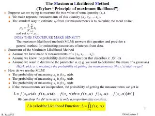
The M aximum L ikelihood M ethod (Taylor: “Principle of maximum likelihood”). l Suppose we are trying to measure the true value of some quantity ( x T ). u We make repeated measurements of this quantity { x 1 , x 2 , … x n }.

E N D
The Maximum Likelihood Method (Taylor: “Principle of maximum likelihood”) l Suppose we are trying to measure the true value of some quantity (xT). u We make repeated measurements of this quantity {x1, x2, … xn}. u The standard way to estimate xT from our measurements is to calculate the mean value: and set xT = mx. DOES THIS PROCEDURE MAKE SENSE??? The maximum likelihood method (MLM) answers this question and provides a general method for estimating parameters of interest from data. l Statement of the Maximum Likelihood Method u Assume we have made N measurements of x {x1, x2, … xn}. u Assume we know the probability distribution function that describes x: f(x, a). u Assume we want to determine the parameter a. (e.g. we want to determine the mean of a gaussian) MLM: pick a to maximize the probability of getting the measurements (the xi's) that we got! l How do we use the MLM? u The probability of measuring x1 is f(x1, a)dx u The probability of measuring x2 is f(x2, a)dx u The probability of measuring xn is f(xn, a)dx u If the measurements are independent, the probability of getting the measurements we got is: We can drop the dxn term as it is only a proportionality constant. P416 Lecture 5
u We want to pick the a that maximizes L: u Often easier to maximize lnL. Both L and lnL are maximum at the same location. we maximize lnL rather than L itself because lnL converts the product into a summation. The new maximization condition is: na could be an array of parameters (e.g. slope and intercept) or just a single variable. n equations to determine a range from simple linear equations to coupled non-linear equations. l Example: u Let f(x, a) be given by a Gaussian distribution function. u Let a = m be the mean of the Gaussian. We want to use our data+MLM to find the mean, m. u We want the best estimate of a from our set of n measurements {x1, x2, … xn}. u Let’s assume that s is the same for each measurement. u The likelihood function for this problem is: gaussian pdf P416 Lecture 5
We want to find the a that maximizes the log likelihood function: u If s are different for each data point then a is just the weighted average: factor out s since it is a constant don’t forget the factor of n Average! Weighted Average P416 Lecture 5
lExample: Poisson Distribution u Let f(x, a) be given by a Poisson distribution. u Let a = m be the mean of the Poisson. u We want the best estimate of a from our set of n measurements {x1, x2, … xn}. u The likelihood function for this problem is: u Find a that maximizes the log likelihood function: Some general properties of the Maximum Likelihood Method JFor large data samples (large n) the likelihood function, L, approaches a Gaussian distribution. J Maximumlikelihood estimates are usually consistent. For large n the estimates converge to the true value of the parameters we wish to determine. J Maximum likelihood estimates are usually unbiased. For all sample sizes the parameter of interest is calculated correctly. JMaximum likelihood estimate is efficient: the estimate has the smallest variance. J Maximum likelihood estimate is sufficient: it uses all the information in the observations (the xi’s). J The solution from MLM is unique. L Bad news: we must know the correct probability distribution for the problem at hand! Average! P416 Lecture 5
Maximum Likelihood Fit of Data to a Function (essentially Taylor Chapter 8) l Suppose we have a set of n measurements: • u Assume each measurement error (s) is a standard deviation from a Gaussian pdf. • u Assume that for each measured value y, there’s an x which is known exactly. • u Suppose we know the functional relationship between the y’s and the x’s: • na, b...are parameters that we are trying determine from our data. • MLM gives us a method to determinea, b... from our data. • lExample: Fitting data points to a straight line. We want to determine the slope (b) and intercept (a). u Find a and b by maximizing the likelihood function L likelihood function: two linear equations with two unknowns P416 Lecture 5
For the sake of simplicity assume that all s’s are the same (s1= s2= si=s): We now have two equations that are linear in the unknowns a, b: in matrix form These equations correspond to Taylor’s Eq. 8.10-8.12 P416 Lecture 5
l EXAMPLE: A trolley moves along a track at constant speed. Suppose the following measurements of the time vs. distance were made. From the data find the best value for the speed (v) of the trolley. u Our model of the motion of the trolley tells us that: u We want to find v, the slope (b) of the straight line describing the motion of the trolley. u We need to evaluate the sums listed in the above formula: best estimate of the speed d0 = 0.8 mm best estimate of the starting point P416 Lecture 5
The MLM fit to the data for d=d0+vt The line in the above plot “best” represents our data. Not all the data points are "on" this line. The line minimizes the sum of squares of the deviations (d) between a line and our data (di): di=data-prediction= di-(d0+vti) →minimize: Σ[di2]→ same as MLM! Often we call this technique “Least Squares” (LSQ). LSQ is more general than MLM but not always justified. P416 Lecture 5